Tuesday, December 1, 2015

Organic Nanopores in Shale


  • Organic Nanopores Structure Materials - Pyrobitumen

The carbon-rich residue of catagenesis, pyrobitumen constitutes the material of organic part of the rock. The Pyrobitumen is a type of solid, amorphous organic matter, which is insoluble to organic solvent (different from bitumen). However, one should not confuse pyrobitumen with residual kerogen in a mature source rock and the distinction is based on microscopic evidence of fluid flow within the rock fabric and is usually not determined. The thermal processes (bitumen to pyrobitumen) driving the molecular cross-linking also decrease the atomic ratio of hydrogen to carbon from greater than one to less than one and ultimately to approximately one half.


  • Gas Adsorption
Similar to surface tension, adsorption is a consequence of surface energy. In a bulk material, all the bonding requirements (be they ionic, covalent, or metallic) of the constituent atoms of the material are filled by other atoms in the material. However, atoms on the surface of the adsorbent are not wholly surrounded by other adsorbent atoms and therefore can attract adsorbates. The exact nature of the bonding depends on the details of the species involved, but the adsorption process is generally classified as physisorption (characteristic of weak van der Waals forces) or chemisorption (characteristic of covalent bonding). It may also occur due to electrostatic attraction.


Affecting Factors: (i) In general, easily liquefiable gases e.g., CO2, NH3, Cl2 and SO2 etc. are adsorbed to a greater extent than the elemental gases e.g. H2, O2, N2, He etc. (while chemisorption is specific in nature.) 

(ii) Porous and finely powdered solid e.g. charcoal, fullers earth, adsorb more as compared to the hard non-porous materials. Due to this property powdered charcoal is used in gas masks.

However, most importantly, the extent of adsorbate adsorption depends directly upon the surface area of the adsorbent.

Adsorption forces and potentials: Methane is generally considered as non-polar molecules. The inter-molecular forces between gas molecules and nanopore surface can be obtained using atom–atom pair potentials, namely a Lennard–Jones (LJ) potential.

[\V_{LJ} = 4\varepsilon \left[ \left(\frac{\sigma}{r}\right)^{12} - \left(\frac{\sigma}{r}\right)^{6} \right] = \varepsilon \left[ \left(\frac{r_{m}}{r}\right)^{12} - 2\left(\frac{r_{m}}{r}\right)^{6} \right]
\]


where ε is the depth of the potential well, σ is the finite distance at which the inter-particle potential is zero, r is the distance between the particles, and rm is the distance at which the potential reaches its minimum.

The r−12 term, which is the repulsive term, describes Pauli repulsion at short ranges due to overlapping electron orbitals and the r−6 term, which is the attractive long-range term, describes attraction at long ranges (van der Waals force, or dispersion force).

Isotherm models: Irving Langmuir was the first to derive a scientifically based adsorption isotherm in 1918. The model applies to gases adsorbed on solid surfaces. It is a semi-empirical isotherm with a kinetic basis and was derived based on statistical thermodynamics. It is the most common isotherm equation to use due to its simplicity and its ability to fit a variety of adsorption data. The mono-layer assumption is addressed by the BET isotherm for relatively flat (non-microporous) surfaces.

Sunday, November 22, 2015

Surface Tension Change with Salinity

Yes, adding salt to water does increase the surface tension of water, although not by any significant amount. 

It is a very common misconception that salt is a surfactant, i.e. a compound that either lowers or breaks surface tension. However, experiments done with salt water show that surface tension actually increases when salt is added to pure water. 

As you know, sodium chloride, or NaCl, is a strong electrolyte, which means it completely dissociates into sodium cations, Na+, and chloride anions, Cl, when placed in water.

http://chem.wisc.edu/deptfiles/genchem/sstutorial/Text7/Tx75/tx75.htmlhttp://chem.wisc.edu/deptfiles/genchem/sstutorial/Text7/Tx75/tx75.html

It turns out that the strong interactions between the sodium cations and the partial negative oxygen, and the chloride anions and the partial positive hydrogens, although they disrupt part of the hydrogen bonding that takes place between water molecules, actually strengthen the surface tension of water.

In other words, you get some ionic component to the overall hydrogen bond-dominated interactions from the addition of these cations and anions. 

A very common experiment meant to illustrate this concept is done by placing salt water drops on a penny. I'll post a link to a great article on such an experiment performed by Lucas Cherkewski

Tuesday, November 3, 2015

Statoil to build the world’s first floating wind farm: Hywind Scotland

Statoil has made the final investment decision to build the world’s first floating wind farm: The Hywind pilot park offshore Peterhead in Aberdeenshire, Scotland.

Sunday, September 20, 2015

Partnership to Take Rock-Fluid Research to the Atomic Level

A partnership between FEI Company and the University of Wyoming (UW) will enable for the first time ever the study of interactions between fluid and rocks at the atomic level for oil and gas research. The research – which aims to advance digital rock technology to achieve a better understanding of the fundamental forces at play in rock-fluid behavior – could potentially impact the entire oil and gas life cycle, from better well design for production to more effective enhanced oil recovery techniques for mature fields.

 - See more at: 
http://www.rigzone.com/news/oil_gas/a/140670/Partnership_to_Take_RockFluid_Research_to_the_Atomic_Level#sthash.wZ8dKwE6.dpuf

Wednesday, August 5, 2015

Mud to Lime: transitional lithotypes


Chalk vs Limestone vs Marble

Chalk is formed in a deep marine environment from the shells of microscopic algae which flourish near the surface, but die and fall to the seafloor. The kind of chalk used in old-style classrooms and lecture theatres scrapes off a thin layer of fine white dust as they are scraped over the abrasive surface of a "blackboard".

Limestone is formed in a shallower marine environment from the bodies of corals and shells, as well as the shells of microscopic sea life. Since it contains large lumps, it does not form such a fine white powder as chalk.

Marble is metamorphosed limestone, ie subjected to heat and pressure, the crystals grow and interlock, forming a stronger rock, more suitable for a building material. Sometimes minerals in the original limestone are still visible as swirls of colour in the marble.


Tuesday, July 7, 2015

Excel VBA

String:
  • chr(13) = change to the next line
  • _ =  break code to two lines


Function:

  • Transpose: Application.WorksheetFunction.Transpose()
  • Upper and lower bound: UBound() and LBound()
  • Join/concatenate: joins text, numbers, cell references, or a combination of those items into one text string
Range:
  • Range("B1:B10 , A4:D6").Select 选中两块不连续区域;
  • Range("B1:B10   A4:D6").Select 选中交叉的区域;
  • Range("B1:B10","A4:D6").Select 选中包含两块区域的最小矩形。


  • UsedRange: 所有使用过的单元格围成的区域;
  • Current Region: 所在的当前的区域;
  • Offset: 向下向右移动位置;
  • Range("A65536").End(xlUp).Offset(1,0): A列第一个非空的单元格;
  • Count: 单元格个数;
  • Address: 单元格位置;
  • Select, Activate
  • Clear, ClearContents, ClearComments, ClearFormats
  • Copy, Cut, Delete


Tuesday, June 30, 2015

Mudrock composition

Mudrocks, by definition, consist of at least fifty percent mud-sized particles. Specifically, mud is composed of silt-sized particles that are between 1/16 – 1/256 of a millimeter in diameter, and clay-sized particles which are less than 1/256 millimeter.

Mudrocks contain mostly clay minerals and quartz ($S_{i}O_{2}$)and feldspars (a group of minerals including aluminum silicates of soda (sodium oxide), potassium (potassium oxide), or lime (calcium oxide)). They can also contain the following particles at less than 63 micrometres: calcite ($CaCO_{3}$), dolomite ($CaMgCO_{3}$), siderite ($FeCO_{3}$), pyrite ($FeS_{2}$), marcasite ($FeS_{2}$), heavy minerals, and even organic carbon.

The term "mudrock" allows for further subdivisions of siltstone, claystone, mudstone, and shale. For example, a siltstone would be made of more than 50-percent grains that equate to 1/16 - 1/256 of a millimeter. "Shale" denotes fissility, which implies an ability to part easily or break parallel to stratification. Siltstone, mudstone, and claystone implies lithified, or hardened, detritus without fissility.

TypeMin grainMax grain
Claystone0 µm4 µm
Mudstone0 µm64 µm
Shale0 µm64 µm
Siltstone4 µm64 µm
Slatenana

Sunday, June 21, 2015

Turbulence Models

Turbulence:
Due to the high degree of mixing, turbulent flow exists. The heat and mass transfer rates are high and can not be explained by molecular transport only. It was seen as a random process in attempt to be specified in statistical parameters. Yet, it is not completely random.

Turbulence is normally expressed in terms of velocity. So there are extras terms in N-S equations, called Reynolds stress, described in terms of turbulence viscosity. This eddy viscosity is a strong function of the distance from the wall, where the eddy diminishes.

In turbulent flow, the kinetic energy imparted to the flow is dissipated into smaller eddies, and finally all the energy dissipated as thermal energy. Two sets of equations in CFD simulation are added to address the conservation of turbulence kinetic energy, $k$, and the turbulent energy dissipation rate, $\varepsilon$.

Prandtl Mixing Length:
When two eddies come closer, they are mixed. The mean distance between eddies is called the "mixing length", which analogous to the mean-free path in gases. The mixing length is a function of distance to the wall.

Friday, June 19, 2015

Model and Simulation: Laws of Conservation

Equation of Continuity:
For 2D incompressible fluid flow from mass conservation,

\[ \frac{\partial v_{x}}{\partial x}+\frac{\partial v_{y}}{\partial y}=0
\]

Thus,

\[ v_{y}=\int_{0}^{y}\frac{\partial v_{x}}{\partial x}dy
\]

Cauchy-Riemann Equation:
Define velocity by new variables, $Psi$, stream function and $phi$, velocity potential,

\[ v_{x}=-\frac{\partial\Psi}{\partial y}
\]

\[ v_{y}=\frac{\partial\Psi}{\partial x}
\]

\[ v_{x}=-\frac{\partial\phi}{\partial x}
\]

\[ v_{y}=-\frac{\partial\phi}{\partial y}
\]


An analytical function $w(z)$ of a complex variable, z, may be chosen such that

\[ w(z)=\phi(z)+i\Psi(z)
\]

satisfying above equations. Velocities can be obtained as the real and imaginary parts of the equation,

\[ \frac{dw}{dz}=-v_{x}+iv_{y}
\]

Equations of continuity, stream function and velocity function in different coordinates are shown below.


Navier-Stokes Equations:
Momentum transport:
\[ \rho\left(\frac{\partial v_{x}}{\partial t}+v_{x}\frac{\partial v_{x}}{\partial x}+v_{y}\frac{\partial v_{x}}{\partial y}+v_{z}\frac{\partial v_{x}}{\partial z}\right)=-\frac{\partial p}{\partial x}+\mu\left[\frac{\partial^{2}v_{x}}{\partial x^{2}}+\frac{\partial^{2}v_{x}}{\partial y^{2}}+\frac{\partial^{2}v_{x}}{\partial z^{2}}\right]+\rho g_{x}
\]

\[ \rho\left(\frac{\partial v_{y}}{\partial t}+v_{x}\frac{\partial v_{y}}{\partial x}+v_{y}\frac{\partial v_{y}}{\partial y}+v_{z}\frac{\partial v_{y}}{\partial z}\right)=-\frac{\partial p}{\partial y}+\mu\left[\frac{\partial^{2}v_{y}}{\partial x^{2}}+\frac{\partial^{2}v_{y}}{\partial y^{2}}+\frac{\partial^{2}v_{y}}{\partial z^{2}}\right]+\rho g_{y}
\]

\[ \rho\left(\frac{\partial v_{z}}{\partial t}+v_{x}\frac{\partial v_{z}}{\partial x}+v_{y}\frac{\partial v_{z}}{\partial y}+v_{z}\frac{\partial v_{z}}{\partial z}\right)=-\frac{\partial p}{\partial z}+\mu\left[\frac{\partial^{2}v_{z}}{\partial x^{2}}+\frac{\partial^{2}v_{z}}{\partial y^{2}}+\frac{\partial^{2}v_{z}}{\partial z^{2}}\right]+\rho g_{z}
\]

Chemical species in incompressible fluids:
\[ \rho\left(\frac{\partial C_{A}}{\partial t}+v_{x}\frac{\partial C_{A}}{\partial x}+v_{y}\frac{\partial C_{A}}{\partial y}+v_{z}\frac{\partial C_{A}}{\partial z}\right)=D_{AB}\left[\frac{\partial^{2}C_{A}}{\partial x^{2}}+\frac{\partial^{2}C_{A}}{\partial y^{2}}+\frac{\partial^{2}C_{A}}{\partial z^{2}}\right]-r_{A}

\]

Heat transfer:
\[ \rho\left(\frac{\partial T}{\partial t}+v_{x}\frac{\partial T}{\partial x}+v_{y}\frac{\partial T}{\partial y}+v_{z}\frac{\partial T}{\partial z}\right)=k\left[\frac{\partial^{2}T}{\partial x^{2}}+\frac{\partial^{2}T}{\partial y^{2}}+\frac{\partial^{2}T}{\partial z^{2}}\right]-\triangle H_{rxn}
\]

1D momentum balance for an unsteady state model gives,
\[ \rho\left(\frac{\partial v_{x}}{\partial t}+v_{x}\frac{\partial v_{x}}{\partial x}\right)=-\frac{\partial p}{\partial x}+\mu\left[\frac{\partial^{2}v_{x}}{\partial x^{2}}+\frac{\partial^{2}v_{x}}{\partial y^{2}}\right]+\rho g_{x}
\]


Using the incompressible fluid solution of equation of continuity,
\[ \rho\frac{\partial v_{x}}{\partial t}=-\frac{\partial p}{\partial x}+\mu\frac{\partial^{2}v_{x}}{\partial y^{2}}+\rho g_{x}

\]

The solution of 1D model equations are given below.


Boundary Conditions:
Differential equations of second order in spatial coordinates and first order in time require two boundary conditions and one initial condition to describe the system.

BC of the first kind:
The temperature or concentration of chemical species are specified at boundaries. This is also known as Dirichlet condition.

BC of the second kind:
The heat transfer or mass transfer flux is constant, also known as Neumann condition.

\[ q=-k_{f}\frac{\partial T}{\partial x}\mid_{x=0}
\]


BC of the third kind:
The flux is not constant, but the transfer coefficient is constant. Usually described in terms of heat or mass transfer coefficient.

\[ -k_{f}\frac{\partial T}{\partial x}\mid_{x=0}=h(T_{s}-T_{\infty})
\]


Friday, June 12, 2015

Model and Simulation: Physical Laws

Equation of State:
Ideal gas: $pV = RT$
Real gas: Peng-Robinson EOS
\[ p=\frac{RT}{(V-b)}-\frac{\alpha a}{V^{2}+2Vb-b^{2}}
\]

$ a = \frac{0.457235\,R^2\,T_c^2}{p_c} $
$ b = \frac{0.077796\,R\,T_c}{p_c} $
$ \alpha = \left(1 + \kappa \left(1-T_r^{\,0.5}\right)\right)^2 $
$ \kappa = 0.37464 + 1.54226\,\omega - 0.26992\,\omega^2 $
$ T_r = \frac{T}{T_c} $

In terms of compressibility, $Z=PV/(RT)$,  and in polynomial form:

$ A = \frac{a\alpha p}{ R^2\,T^2} $
$ B = \frac{b p}{RT} $
$ Z^3 - (1-B)\ Z^2 + (A-2B-3B^2)\ Z -(AB-B^2-B^3) = 0 $

where $\omega$ is the acentric factor of the species, R is the universal gas constant. Possible roots, 1 three real roots (largest, gas volume; smallest liquid volume); 2 one real (true volume) two imaginary.

The fugacity of pure component is given by,

\[ \ln\phi=\ln\frac{f}{p}=Z-1-\ln(Z-B)-\frac{A}{2\sqrt{2}B}\ln\left(\frac{Z+2.414B}{Z-0.414B}\right)

\]

Mixing rules:
Parameters of PR equation for the mixture of N simple fluids where molar percent of the i-th component is zi are defined by mixing rules

\[ a=\sum_{i}\sum_{j}z_{i}z_{j}a_{ij}
\]

\[ b=\sum_{i}z_{i}b_{i}
\]

where, $a_{ij}=(1-\delta_{ij})\sqrt{a_{i}a_{j}}$

Here aij is expressed through empirically determined binary interaction coefficient δij characterizing the binary formed by component i and component j.

Some δij are tabulated (e.g. table 4.2 in Pedersen and Christensen(2006)). For those one which are not tabulated formula of Chueh and Prausnitz (1967) could be used:

\[ 1-\delta_{ij}=\sqrt{\frac{2V_{c,i}^{1/6}V_{c,j}^{1/6}}{V_{c,i}^{1/3}V_{c,j}^{1/3}}}
\]


Formula for fugacity coefficient of the mixture, calculated via PR equation and standard mixing rules, has expression (see Peng and Robinson (1976) or equation 4.65 in Pedersen and Christensen (2006) for more detail)

\[ \ln\phi_{i}=\ln\frac{f_{i}}{z_{i}p}=\frac{b_{i}}{b}(Z-1)-\ln(Z-B)-\frac{A}{2\sqrt{2}B}\left(\frac{2}{a}\sum_{j}^{N}z_{j}a_{ij}-\frac{b_{i}}{b}\right)\ln\left(\frac{Z+2.414B}{Z-0.414B}\right)
\]

The enthalpy departure of the a fluid is given by,

\[ H-H^{*}=RT(Z-1)+\frac{T\frac{da}{dT}-a}{2\sqrt{2}b}\ln\left(\frac{Z+2.414B}{Z-0.414B}\right)
\]


Henry's Law:
The mole fraction or partial pressure of ith component, $p_i$ is proportional to the mole fraction of ith component in the liquid phase, $x_i$,

\[ p_{i}=H_{i}x_{i}
\]

For ideal gas,

\[ p_{i}=y_{i}P
\]


Thus, a linear equilibrium relationship is obtained,

\[ \frac{y_{i}}{x_{i}}=\frac{H_{i}}{P}
\]

For pure gas adsorption at pressure P, the number of moles adsorbed on the surface, n, is given by Henry's law for adsorption,

\[ n=kP
\]


$H_i$ is Henry constant; $P$ is total pressure; $y_i$ is mole fraction of ith component in vapor phase.

Newton's Law of Viscosity:
The shear stress is proportional to shear rate,

\[ \tau_{yx}=-\mu\frac{dv_{x}}{dy}

\]

All the gases and liquids and solutions of low-molecular-weight compounds exhibit Newtonian behavior. Non-Newtonian behaviors are shown below,


Some dimensionless numbers, such as Prandtl and Schmidt numbers can be obtained for empirical correlations for heat and mass transfer.

Fourier's Law:
Heat transfer rate of conduction due to temperature difference is written as,

\[ \dot{q}=kA\frac{(T_{2}-T_{1})}{\triangle z}=-kA\frac{dT}{dz}

\]

The differentiation form may be used if heat transfer area is a variable,

\[ \frac{d}{dz}\left(A\frac{dT}{dz}\right)=0

\]

Convective heat transfer at low temperature by Newton's law of cooling,

\[ \dot{q} = hA(T_2 - T_1)
\]

$k$ is the thermal conductivity; and $h$ is the heat transfer coefficient.

Fick's First Law:
For steady-state diffusion without convection, Fick's first law applies. The molar flux is described as,

\[ J_{A}=-CD_{AB}\nabla x_{A}\underrightarrow{C\,is\,constant}-D_{AB}\nabla C_{A}\underrightarrow{1-D}-D_{AB}A\left(\frac{dC_{A}}{dz}\right)

\]


where, $D_{AB}$ is the diffusion coefficient of A in B; $J_A$ is the molar flux of A; $C_A$ is the molar concentration of A; $x_A$ is the mole fraction of A.

Or the Fick's law gives the diffusive flux relative to the average velocity of fluid mixture. In absence of convection, the diffusive flux and the total flux are the same. For diffusion relative to fixed/stationary coordinates, the molar flux becomes,

\[ N_{A}=J_{A}+vC_{A}=-C_{A}D_{AB}\nabla x_{A}+v^* C_{A}
\]

where, average velocity, $v^*$ is $x_A v_A + x_B*v_B$.

\[ N = N_A + N_B = Cv^* = C_A v_A + C_B v_B
\]

Since the mass transfer results in some amount of convection (diffusional flux), the first law is valid only for dilute solutions or in cases of diffusion in solids. In concentrated solutions, the diffusion coefficient depends on the concentration.

Fick's Second Law:
It describes how diffusion causes the concentration to change with time.

\[ \frac{\partial C}{\partial t}=D_{AB}\frac{\partial C^{2}}{\partial z^{2}}

\]

Film Model:
The assumptions for film theory:
  1. The entire variation of concentration or temperature takes place within a thin fluid film adjacent to the interface. While, in the bulk fluid, the concentration or temperature is almost uniform.
  2. Within the film, the mass or heat transfer takes place by steady-state 1-D diffusion or conduction, respectively.
The mass transfer flux for species A is written in terms of diffusion coefficient, concentrations at the two faces of the fictitious film and film thickness,

\[ N_{A}=D_{AB}\frac{\left(C_{A2}-C_{A1}\right)}{\delta_{m}}

\]

Note that $C_{A2}$ is same as the concentration in bulk flow.

But in terms of mass transfer rate, $k$, which is measurable by experiment,

\[ N_{A}=k(C_{A2}-C_{A1})

\]

Differently, the mass transfer coefficient depends on the hydrodynamics, i.e. the fluid flow field in the bulk fluid.

Thus, the film thickness can be obtained,

\[ \delta_{m}=\frac{D_{AB}}{k}

\]

Two-Film Theory:
For two-phase flow, the mass transfer across the interface can be simplified:

  1. The resistance to mass transfer lies in two different fictitious films adjacent to the interface on both of its sides.
  2. The concentration of the chemical species in both phase at the interface is in equilibrium (insignificant mass transfer across the interface).

The total mass transfer coefficients $K_g$ and $K_l$ can be expressed in term of the individual mass transfer coefficient (when Henry's law applies):

\[ \frac{1}{K_{g}}=\frac{1}{k_{g}}+\frac{H}{k_{l}}
\]

\[ \frac{1}{K_{l}}=\frac{1}{k_{l}}+\frac{1}{Hk_{g}}

\]

If the mass transfer in the liquid phase is controlling, then kg>>kl and hence $K_l=k_l$. Vice versa.

Similarly, this also applies to heat transfer, where constant temperatures are canceled.

\[ \frac{1}{U}=\frac{1}{h_{1}}+\frac{1}{h_{2}}
\]


Arrhenius' Law:
The chemical reaction rate can be the product of two terms, one depends on concentration (associated with pressure terms) and one depends on temperature only.

\[ -r_{A}=f\left(C_{A},C_{B},...\right)k^{'}(T)
\]

The temperature term can be written as follows, Arrhenius' Law,
\[ k^{'}(T)=k_{0}^{'}e^{-E/RT}
\]

$k^{'}$ is the kinetic rate expression; $k_0^{'}$ is the constant, E is the activation energy of the reaction.

Adsorption Isotherms:
The equilibrium relationship relating $q$ (the mount adsorbed on the solid) and $C_A$ (the concentration of the adsorbate in the fluid)  is known as Isotherm. Sometimes, isotherms are given in terms of $K = K_a / K_d$ (rates of adsorption and desorption) and $\theta = q / q_0$ ($q_0$ is the adsorption capacity of adsorbent). Commonly used adsorption isotherms are,


  • Langmuir (1918), no interaction between the adsorbed molecules

\[ p=\frac{1}{K}\left(\frac{\theta}{1-\theta}\right)
\]
  • Brunauer-Emmett-Teller (1938), $p_{r}=p/p_{s}$, $q_m$ = constant
\[ \frac{q}{q_{m}}=\frac{K_{B}p_{r}}{(1-p_{r})(1-p_{r}+K_{B}p_{r})}
\]

  • Freundlich (1926) Empirical

\[ q=k_{F}C^{1/n_{F}}

\]

  • Raddke and Prausnitz (1972) combines Freundlich isotherms and Henry's law

\[ q=\frac{1}{\left(\frac{1}{K_{Hp}}+\frac{1}{k_{F}p^{1/n_{F}}}\right)}

\]

References:
Verma, Ashok Kumar. 2014. Process Modelling and Simulation in Chemical, Biochemical and Environmental Engineering. CRC Press.

http://en.wikipedia.org/wiki/Equation_of_state

http://kshmakov.org/fluid/note/3/

Wednesday, June 10, 2015

Model and Simulation: Simplifications in Model

Model Simplification:

Continuum: Laws of conservation hold in continuous phase. For dispersed bubble or solid particles in liquid, if the main mechanism is away from the interface of the dispersed and continuous phases, it may be convenient to consider the entire dispersion to be a continuous phase, e.g. study on the pipe wall and pressure loss. If the main mechanism takes place at the gas-liquid interface, continuum is meaningless, e.g. mass transfer between the bubble and liquid.

Combining simple and rigorous models: Two ways to model dispersed bubble in liquid, 1. build rigorous cell model for the dispersed bubble and surrounding liquid, and combine them in a simple manner. 2. Apply simple thin film model at the surface of the bubble and combine with the mass transfer and bubble-size distribution in a rigorous manner.

Uniform Probability Distribution: Useful in averaging the properties assuming the individual entity follow uniform distribution law, e.g. in adsorption, the probability of occupying the empty space on the surface is the same.

Parallel Mechanisms: The mechanism of  heat transfer is conduction, convection and radiation due to molecular motion, bulk flow and infrared radiation. The parallel mechanism allows us to treat different mechanisms separately, but under the assumption that there is no interaction between different mechanisms.

Analogy to Electrical Circuits: Many transport mechanisms are analog to the flow of current in electrical circuits.
Current flow: Ohm's Law;
Heat transfer: Fourier's Law;
Mass transfer: Fick's Law.
(Heat transfer due to radiation is described by Stephan-Boltzman's Law, i.e., the rate of heat transfer is proportional to the difference of the fourth power of the temperature.)

Film Model and Boundary Layer Approximation: The film model uses the assumption that in the small region adjacent to the wall, the variation is much larger than that at the center. Thus the concept of thin film at the wall is developed and accounts for all the variations. The central cylinder is considered with no variation.
But the boundary layer model allows the layer thickness to vary with time and distance. It is more likely an approximation to the reality, the experimental results.

Order of magnitude Approximation: If the ratio of the contribution from one mechanism and that from others is high enough, then the other mechanisms can be neglected to reduce the complexity.

Quasi-Steady State: The assumption for unsteady-state problem, that during a small time interval, the process is at steady-state is known as "quasi-steady state".

Finite and infinite dimensions: Many mathematical equations approach certain value when one or some of its parameters goes to infinity or zero, which is not possible in physical experiments. Thus, it can be assumed that when the parameter value is large or small enough, it is close to infinity or zero.

References:
Verma, Ashok Kumar. 2014. Process Modelling and Simulation in Chemical, Biochemical and Environmental Engineering. CRC Press.

Tuesday, June 9, 2015

Model and Simulation: Equations

Equations describe the interrelations between various parameters.

Algebraic Equation:

  • Linear equation, solved by matrix inversion
  • Non-linear equation, solved by linearisation or non-linear optimization

A non-linear equation $ F(\vec{x})=\vec{0}$ can be written by

\[ F(\vec{x})=\vec{R}
\]

where, $\vec{x}$, $\vec{0}$ and $\vec{R}$ are vectors.

R are the residuals and the objective function becomes $|\vec{R}|$, which is to be minimized.

By linearisation, the set of non-linear equations can be converted to,

\[ F_{i}(\vec{x})=-\sum_{j}J_{ij}(\vec{x})\triangle x_{j}
\]

where, $J_{ij}(\vec{x})=\frac{\partial F_{i}(\vec{x})}{\partial x}$.

An initial guess is required to start this iterative solving process. The Jacobian matrix is estimated using the values of x from the previous iteration until the right-hand side becomes less than the tolerance.

Various optimization methods can be used to search the optima within a given range. The problems can be

  1. The obtained optima is local optima or there are multiple optima -- Genetic Algorithm, Simulated Annealing
  2. The solution won't converge or stick at particle values -- try different methods or change the initial guess
Again, the choice of initial guess is very important.


Differential Equations:
If only one type of derivative is involve, the equation is called ODE, ordinary differential equation, as opposed to PDE, partial differential equation.

A Cauchy problem in mathematics asks for the solution of a partial differential equation that satisfies certain conditions which are given on a hypersurface in the domain. A Cauchy problem can be an initial value problem (given initial value, how the system evolves with time) or a boundary value problem (specifying the boundary condition instead), but it can be none of them. Cauchy boundary conditions require both the function value and normal derivative on the boundary of the domain (a Dirichlet and a Neumann boundary condition) to ensure a unique solution.

Sometimes, PDEs are converted into simultaneous ODEs or algebraic equations (a large system of coupled ODEs with derivatives with respect to time). When the phenomena vary with time, the spatial variables are discretised and time is considered a continuous variable. Such as parabolic and hyperbolic equations in unsteady-state models. This method is termed a "method-of-line".

In steady state models, spatial discretisation results in algebraic equations. Such as elliptic equations.


Differential-Algebraic Equations:

DAEs, these types of mixed equations contain unsteady-state material and energy balance equations, equilibrium relationships, consistency equations etc.


Other Equation Type Classification:

Homogeneous Function:
If x is the solution of the function, so is $\lambda x$.
\[ f(\lambda x)=\lambda^{n}f(x)
\]


Homogeneous linear differential equations:
 If  $\phi(x)$  is a solution, so is  $c \phi(x)$. In another word, each term in a linear differential equation must contain y or any derivative of y, such as $ \sin(x) \frac{d^2y}{dx^2} + 4 \frac{dy}{dx} + y = 0 $.

Second order differential equations:

\[ Au_{xx} + 2Bu_{xy} + Cu_{yy} + Du_x + Eu_y + F = 0
\]

If $B^2 - AC > 0$, hyperbolic partial differential equation;
If $B^2 - AC = 0$, parabolic PDE;
If $B^2 - AC < 0$, elliptic PDE.

The most famous wave equation is a hyperbolic PDE. In one spatial dimension, this is $u_{tt} - u_{xx} = 0$.

Source of Equations:
The source of the equations depends on the field of application and the knowledge of the modeler.

Empirical Equations:
These can be obtained by fitting the experimental data in terms of important parameters with somem simple functions. The relation can explicit or implicit (friction factor by McCable et al. 1993).

Based on theoretical concepts:
Such as the calculation/estimation of thermodynamic properties.

Consistency Equations:
Based on the fact that the fractional composition of each component should add up to 1, in terms of mole and mass.

Law of conservation:
Such as equation of continuity and the momentum-balance equation with considerations of energy/mass generation or depletion in chemical reaction, viscous dissipation, electrical or electrochemical effects on the flow and other phenomena. The generalized equation of change is known as the Navier-Stokes equation.

Integration/Averaging:
Flow rate is obtained by integrating the velocity over the cross-sectional area;
Average velocity is then obtained by division of the total area.
Also, number-averaged particle diameter, porosity...

Population Balance:
Discrete event model considers the birth and death of population (breakage, agglomeration or coalescence).

References:
Verma, Ashok Kumar. 2014. Process Modelling and Simulation in Chemical, Biochemical and Environmental Engineering. CRC Press.

Monday, June 1, 2015

Models and Simulation - Types of Models

Types of Models:
Three major model types are deterministic model, discrete-event model and stochastic model.

  • Deterministic Models: No random variable;
  • Lumped Parameter Models: ODE, all spatial distributions are lumped into one variable;
  • Distributed Parameter Models: PDE, consisting of spatial derivatives;
  • Steady-State/Static Models: No temporal derivative;
  • Unsteady-State/Dynamic Models: With temporal derivatives;
  • Stochastic Models: Random variables involved (probability distribution function/pseudo-random numbers)
  • Population Balanced Models: In multiphase system, discrete/dispersed phases are present as particles, droplets or bubbles. Similar to the "birth and death" of individuals, the particles can agglomerate or break and the bubbles and droplets can break and coalesce. Thus, the number of identities of discrete phases, called population, and the size of the individuals change and form a particle/droplet/bubble-size distribution.
  • Agent-Based Models: Each part of the model , called an agent, is capable of making decisions with strong human behavior involved;
  • Discrete-Event Models: The states, even time, are considered discrete and NON-continuous;
  • Artificial Neural Network-based Models: A black-box approach to correlate various parameters and then predict outcomes from information available. No exact relation between the inputs and outputs is almost possible to establish. No contribution to the understanding of the phenomena.
  • Fuzzy Models: based on fuzzy mathematics or fuzzy logic involving fuzzy variables. Fuzzy, not well quantified, such as small, large, very large.


-- The general-purpose language/software can handle various types of models/problems, but require coding of the model equations using the syntax and semantics of the software. While, more dedicated software generates an appropriate set of models of equations for the users to use, but the scope is limited.

-- Stochastic Models:
The random numbers are characterized by their moment. The first moment is known as "average" or "expectation". A model may consider only average properties, thus avoiding the complexity of the process due to the randomness of the properties. Many models consider random behavior of the parameters, although the outputs of the model are average properties. These models also are probabilistic in nature. Various moments of the random variables may be determined analytically (Coulomb's Law?) or by Monte Carlo simulation. The random variables follow a probability distribution function. The choice of the distribution is determined from the assumption involved.

References:
Verma, Ashok Kumar. 2014. Process Modelling and Simulation in Chemical, Biochemical and Environmental Engineering. CRC Press.

Friday, May 15, 2015

Osmotic Pressure Calculation

By thermodynamics, the chemical potential of solvent (water) in a solution containing pure solvent and solute is expressed as,

\[ \mu_{w}\left(l,x_{w},p+\pi\right)=\mu_{w}^{0}\left(l,p+\pi\right)+\nu RT\ln a_{w}
\]

where, $\mu_w$ is the chemical potential of solvent, which is a function of solvent, $l$, mole fraction of solvent $x_w$, external pressure, $p$, and additional osmotic pressure exerted by solutes, $\pi$ (whereas, for the pure solvent, $x_w$ goes away); $\nu$ is the dissociation coefficient (a solute dissociates into $\nu$ ions); $R$ is the gas constant; $T$ is temperature in consistent with $R$; $a_w$ is water activity.

The addition to the pressure is expressed through the expression for the energy of expansion:

\[ \mu_{w}^{o}(l,p+\pi)=\mu_{w}^{0}(l,p)+\int_{p}^{p+\pi}V\mathrm{d}p
\]


where, $V$ is the molar volume of solvent.

To balance the chemical potentials of solvent for two solutions with and without solute separated by semipermeable membrane, $\mu_{w}\left(l,x_{w},p+\pi\right)$ and $\mu_{w}\left(l,p\right)$,

\[ -\nu RT\ln a_{w}=\int_{p}^{p+\pi}V\mathrm{d}p

\]

Thus, osmotic pressure is expressed as opposed to pure solvent (water), in which water activity is 1,

\[ \pi=-\nu RT/V\ln a_{w}

\]

Conventionally, the gradient of osmotic pressure is approximated using the concentration or the mass fraction of solute (salt). The derivation is shown as follows.

A definition of water activity is,

\[ a_{w}=l_{w}x_{w}=l_w(1-x_s)
\]


where, $l_w$ is activity coefficient; and $x_w$ is the mole fraction of water in aqueous fraction ($x_s=1-x_w$ is the mole fraction of solute). By Raoult's law, $l_w$ is usually approximated as unity in dilute solution.

Using Taylor series, $\ln l_w(1-x_s) \approx -x_s$.

Thus, the osmotic pressure becomes ($C$ is the molar concentration of solute),

\[ \pi=-\nu RT/V\ln a_{w} = \nu RT/V x_s = \nu RT C

\]


Also, the relation between the gradients of osmotic pressure and chemical potential is,

\[ \nabla\pi=-\frac{1}{V}\cdot\nabla\mu_{w}

\]

The relation between the gradient of osmotic pressure and the concentration or the mass fraction of solute (salt) becomes,

\[  \nabla\pi\approx\nu RT\nabla C=\nu RT\frac{\rho}{M_{s}}\nabla X
\]


where, $\rho$ is the solution density; $M_s$ is molar mass of solute; and $X$ is the mass fraction of solute.

Monday, March 23, 2015

Effects of Cryogenic Fluids as A Fracturing Fluid - T. Patterson defense

233 bans or severe hindrances in municipalities across US
See www.foodandwaterwatcj.org/water/fracking

Non-water-based fracking
1. Gelled liquid CO2 (Gupta, 1998)
2. Cryogenic (Grundman, 1998)


Saturday, March 14, 2015

Determine the rock mechanic properties for paleo-times

Example from William Fork in Piceance Basin from Cumella and Scheevel, 2008

Evidences to determine the rock mechanic properties in paleo-times, whether it behaves elastically or not, can include:
  • Present rock strain-recovery test see if it is elastic recovery.
  • Determine the time span for the study, whether it is short or long time. For example, natural fractures generated during gas generation by coal.
  • Low or negligible thermal effects
If the time span of the study in the paleo-times is relative short and present strain-recovery is elastic from core test, it can be assumed that the rock behaved elastically during that time span. Otherwise, non-elastic effects can play a role, such as pressure-solution, which can dissipate the stress during that process and result in non-elastic behavior.

Thursday, March 12, 2015

Unit Conversion Coefficients in oil and gas engineering equations

Flow Rate Conversion:

According to,
\[ 1 m^3/s = 543440 bbl/day
\]

\[ 1 cm^3/hr = (543440)(10^{-6})/3600 bbl/day
\]

Thus,

\[ 1 bbl/day = (3600)(10^6)(543440) = 6624.46 cm^3/hr
\]

Alternatively,

\[ 1 bbl  = 0.158987 m^3
\]

Thus,

\[ 1 bbl/day = (0.158987)(10^6)/(24) = 6624.46 cm^3/hr
\]

If the fluid is water with density of $1 g/cm^3$,

\[ 1 bbl/day = 6624.46 g/hr
\]

Multiply specific gravity, SG, to covert to other fluids.

Darcy Equation Radial Flow:

\[ q_{well}=-0.006328\frac{2\pi kh\left(p_{e}-p_{well}\right)}{B\mu\ln\left(r_{1}/r_{w}\right)}=-0.039765\frac{kh\left(p_{e}-p_{well}\right)}{B\mu\ln\left(r_{1}/r_{w}\right)}
\]

where, the conversion factor,

\[\frac{[mD][psi]}{[cp]}= \frac{0.9869233 \times 10^{-15} \times 10.7639[ft^2][psi]}{10^{-3} \times 0.000145038 [psi] \frac{1}{60\times 60\times 24}[day]} =  0.006328 \frac{[ft^{2}]}{[day]}
\]

\[ 0.006328\frac{[mD][ft][psi]}{[cp]}=\frac{[ft^{3}]}{[day]}
\]

If using $bbl/day$ instead of $ft^3/day$, $1\,bbl=5.6146\,ft^{3}$.

\[ \frac{0.006328\times2\pi}{5.146}=0.001127\times2\pi=0.007082=\frac{1}{141.2}
\]

thus,

\[ q_{well}=-\frac{kh\left(p_{e}-p_{well}\right)}{141.2B\mu\ln\left(r_{1}/r_{w}\right)}

\]

However, for gas flow, the bottomhole flow rate has to be converted to standard conditions ($T_{sc}=60 F = 520 R$ and $P_{sc} = 14.7 psi$).

\[ q_{g}=\frac{p_{sc}}{T_{sc}}\frac{zT}{p}q_{g,sc}
\]

Substitute in horizontal radial flow equation (steady-state, homogeneous):

\[ \frac{p_{sc}}{T_{sc}}\frac{zT}{p}q_{g,sc}=\frac{0.006328\times\left(2\pi rh\right)k}{\mu}\frac{dp}{dr}

\]

Integrate from wellbore to reservoir boundary:

\[ \frac{Tq_{g,sc}}{kh}\ln\left(\frac{r_{e}}{r_{w}}\right)=0.703\int_{p_{wf}}^{p}\frac{2p}{\mu z}dp

\]

Assume viscosity and z-factor are constant and ensure the unit of $q_{g,sc}$ is in $Mscf/day$ (thousand standard cubic feet per day):

\[ q_{g,sc}=\frac{kh\left(p_{ave}^{2}-p_{wf}^{2}\right)}{1424T\mu z\ln\left(\frac{r_{e}}{r_{w}}\right)}

\]

Diffusivity Equation:

Unit conversion factors of 0.006328 and 0.007082:

According to Darcy's law:

\[ q=0.001127\frac{kA\triangle p}{\mu L}
\]

where, $q$ is in $bbl/day$; $k$ is in $mD$; $\triangle p$ is in $psi$; $\mu$ is in $cp$; $L$ is in $ft$.

Due to the conversion of 1 $bbl$ = 5.6146 $ft^3/day$,

\[ q=(0.001127)(5.6146)\frac{kA\triangle p}{\mu L}=0.006328\frac{kA\triangle p}{\mu L}
\]

For radial flow of incompressible fluids:

\[ v=\frac{q}{A}=0.001127\frac{k}{\mu}\frac{dp}{dr}
\]

where, $A=2\pi rh$. Thus, by integration,

\[ \int_{r_{1}}^{r_{2}}\frac{q}{2\pi rh}dr=0.001127\int_{p_{1}}^{p_{2}}\frac{k}{\mu}dp
\]

Hence,

\[ q=(2\pi)(0.001127)\frac{kh\triangle p}{\mu\ln(r_{2}/r_{1})}=0.007082\frac{kh\triangle p}{\mu\ln(r_{2}/r_{1})}
\]

where, $q$ is in $bbl/day$; $k$ is in $mD$; $\triangle p$ is in $psi$; $\mu$ is in $cp$; $L$ is in $ft$.

Gas Diffusion and Adsorption:

Diffusion Coefficient:

\[ D^{k*}=10^3\frac{b^K k^\infty}{\mu}
\]

where, $D^{k*}$ in $cm^2/s$, $b^K$ in atm, k in mD, $\mu$ in cp = $mPa \cdot s$, so

\[ cm^2/s=10^3\frac{atm \cdot mD}{cp}=10^3\frac{10^5Pa \cdot 10^{-12} m^2}{10^{-3}Pa\cdot s}=10^{-4}m^2/s
\]

Multiply by $(93)$ convert from $cm^2/s$ to $ft^2/day$.

Gas Diffusion: 

Solute Concentration:

Molality:
Also called molal concentration, is a measure of the concentration of a solute in a solution in terms of amount of substance in a specified amount of mass of the solvent.
A commonly used unit is mol/kg. A solution of concentration 1 mol/kg is also sometimes denoted as 1 molal.

The molality ($b$), of a solution is defined as the amount of substance (in $mol$) of solute, $n_{solute}$, divided by the mass (in $kg$) of the solvent, $m_{solvent}$:

\[ b = \frac{n_{solute}}{m_{solvent}}
\]

Molarity:
Molar concentration, also called molarity, amount concentration or substance concentration, is a measure of the concentration of a solute in a solution, or of any chemical species in terms of amount of substance in a given volume. A commonly used unit for molar concentration used in chemistry is mol/L. A solution of concentration 1 mol/L is also denoted as 1 molar (1 M).

Molar concentration or molarity is most commonly expressed in units of moles of solute per litre of solution. For use in broader applications, it is defined as amount of solute per unit volume of solution, or per unit volume available to the species, represented by lowercase $c$:

\[ c = \frac{n}{V} = \frac{N}{N_{\rm A}\,V} = \frac{C}{N_{\rm A}}
\]

Here, $n$ is the amount of the solute in moles, $N$ is the number of molecules present in the volume $V$ (in litres), the ratio $N/V$ is the number concentration $C$, and $N_A$ is the Avogadro constant, approximately $6.022×10^{23} mol^{−1}$.

Or more simply: 1 molar = 1 M = 1 mole/litre.

PPM (parts-per-million):
Parts-per notation is often used describing dilute solutions in chemistry. When working with aqueous solutions, it is common to assume that the density of water is 1.00 $g/mL$. Therefore, it is common to equate 1 gram of water with 1 mL of water. Consequently, $ppm$ corresponds to 1 $mg/L$ and $ppb$ corresponds to 1 $μg/L$.

Conversions:

The conversions to and from the molar concentration, $c$, for one-solute solutions are

\[ c = \frac{\rho\, b}{1+ b M},\ b=\frac{c}{\rho-cM}
\]

where $\rho$ is the mass density of the solution, $b$ is the molality, and $M$ is the molar mass of the solute.

To be exact, ppm is interchangeable with molality solute through molecular weight,

\[ 1 ppm = \frac{10^{3} mol/kg}{M_w}
\]

Because it is usually easier to measure liquids by volume instead of mass, molarity (M) is defined as the number of moles of solute ($n$) divided by the volume ($V$) of the solution in liters. Thus,

\[ 1 ppm = \frac{10^{3} mol/L}{M_w}
\]

This is only valid for dilute solution. As salt concentration increases, the volume of solution varies (larger or smaller) and the deviation enlarges.

Friction Pressure:


Friction Head Loss:

\[
h_{f}=\frac{2f_{f}V^{2}L}{g_{c}d}
\]


where, $f_{f}$ is Fanning Friction Factor, quarter of Moody Factor.

Friction Pressure:

\begin{eqnarray*}
p_{f} & = & \frac{2f_{f}V^{2}\rho L}{d}=\frac{2f_{f}(q/A)^{2}\rho L}{d}=\frac{2f_{f}(\frac{4q}{\pi d^{2}})^{2}\rho L}{d}=2\frac{16}{\pi^{2}}\frac{f_{f}q^{2}\rho L}{d^{5}}\\
& = & 2\frac{16}{\pi^{2}}\frac{\left[bpm\right]^{2}\left[lbm/ft^{3}\right]\left[ft\right]}{[in]^{5}}=2\frac{16}{\pi^{2}}\frac{\left[\frac{5.6146ft^{3}}{60s}\right]^{2}\left[\frac{lbm}{ft^{3}}\right]\left[ft\right]}{[in]^{5}}\\
& = & 2\frac{16}{\pi^{2}}\frac{\left(\frac{5.6146}{60}\right)^{2}\left[ft^{3}\right]\left[lbm\frac{ft}{s^{2}}\right]}{[in]^{5}}=2\frac{16}{\pi^{2}}\left(\frac{5.6146}{60}\right)^{2}\frac{\left(12\right)^{3}\left[lbm\frac{ft}{s^{2}}\right]}{in^{2}}\\
& = & 2\frac{16}{\pi^{2}}\left(\frac{5.6146}{60}\right)^{2}\left(12\right)^{3}\frac{1}{32.174}\frac{lbf}{in^{2}}\\
& = & 1.52484psi
\end{eqnarray*}


Sunday, March 8, 2015

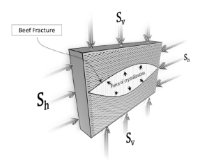
Force of Crystallization - Beef fracture and Nahcolite Nodules

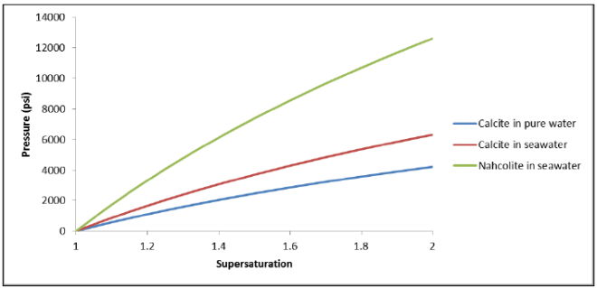
Crystal of Nahcolite → High Crystallization Pressure → Nodules

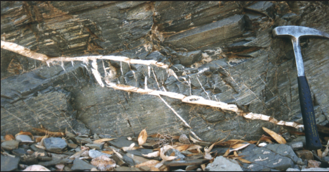
Crystal of Calcite → Lower Crystallization Pressure → Contained within bedding-parallel fractures, grows as vein and forms the beef fractures.
1

Analysis of the force of crystallization for both calcite and nahcolite was presented as a function of the degree of solution supersaturation and the partial molar volume change of the precipitated mineral. The pressure generated from crystal growth of nahcolite is significantly higher than what calcite crystal growth can generate. This implies that crystallization forces significantly exceeding the in-situ stress condition (i.e., the crystals cannot be contained within the vein) create the widely observed large sizes of nahcolite nodules. However, calcite is usually observed as veins, implying that the forces of calcite crystallization are probably contained with the bedding-parallel fractures forming the widely observed beef fractures.

Vein

In geology, a vein is a distinct sheetlike body of crystallized minerals within a rock. Veins form when mineral constituents carried by an aqueous solution within the rock mass are deposited through precipitation.

Fibrous mineral veins generally grow by precipitation from supersaturated aqueous solutions.The force of crystallization as a function of the degree of solution supersaturation (ratio of the actual concentration to the concentration in a normal saturated solution) and the partial molar volume change of the precipitated mineral.

vein

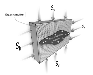
Natural Forces in Fracturing Systems

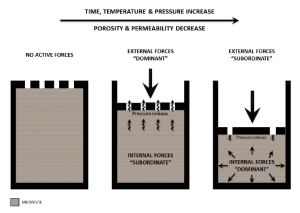
Natural forces acting in a sedimentary basin can be grouped into two categories: (1) external forces and (2) internal forces.

External forces, which are created by sediment load and tectonics, are dominant during early burial.

Continuous pressure release exists, creating equilibrium with a hydrostatic pressure. With subsequent burial, both temperature and pressure increase. However, porosity and permeability decrease. Pressure release is limited because of the limitations of decreasing porosity and permeability. At that point, internal forces, which are caused by clay inter-layer reactions, mineral crystallization or petroleum generation, will dominate.

1

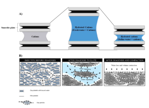
  • Force of clay inter-layer reactions:
    Interaction between swelling clay and water can generate forces that cause rock volume contraction and water expulsion during both early and late diagenesis.

2

  • Force of crystallization:
    The mineral crystallization-generated force is a consequence of precipitation from supersaturated solution and crystal growth causing a rock volume expansion .

3

  • Force of petroleum expulsion:
    The petroleum expulsion-generated force is a consequence of kerogen maturation and petroleum generation causing rock volume expansion.

4

Friday, March 6, 2015

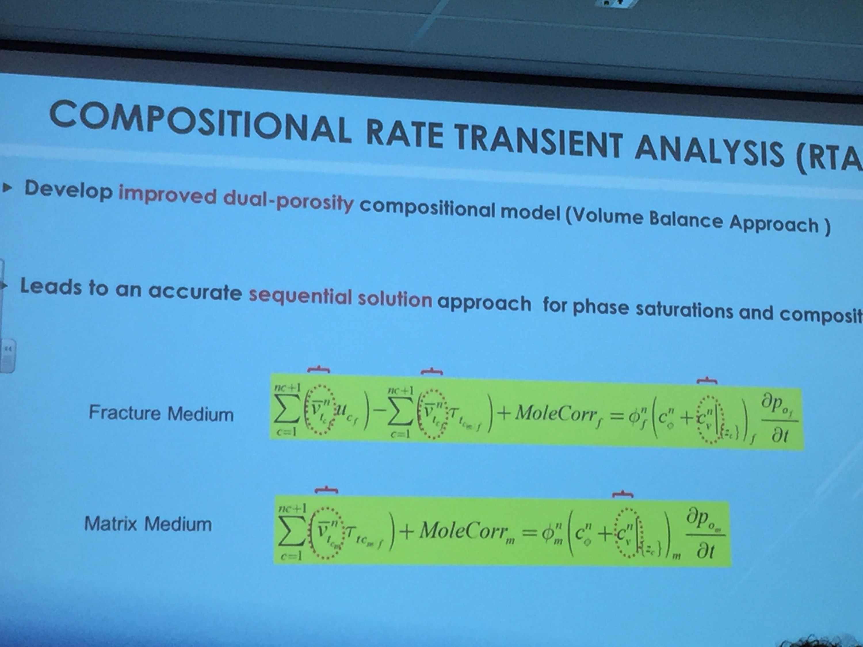
Compositional Modeling and EOR for Liquid Rich Shales

March 6, 2015 Najeeb Defense
  • Compositional Rate Transient Analysis
  • EOR Potential

Driving Forces: Gravity, Darcy and Molecular Diffusion (mostly important but often overlooked). Combined effects (oil swelling effect, viscosity reduction and IFT reduction at Matrix and Fracture interface) were able to match the CO2 soaking experiments for Mid-Bakken. NGL may be better that CO2 for higher RF.

Thursday, March 5, 2015

LyX Longtable

If length of table covers more than one page, use "longtable".

  • Don not use Table Float!

Steps:

  1. Insert a long;

  2. Put cursor to the headline, insert a row below (so two headlines);

  3. Right Click ⇒More⇒Settings⇒Longtable: here, check both of the Headline and Caption;

  4. You will find out one the headlines turn into Caption, insert Label here.

longtable

Wednesday, March 4, 2015

Words and Phrases Translation

March 3, 2015
  • Tasmanites, ['tæzmənait]: 塔斯曼油页岩
  • inasmuch as, 因为

    1. We were doubly lucky inasmuch as my friend was living on the island and spoke Greek fluently.

March 4, 2015
  • meteoric [,mitɪ'ɔrɪk]:  大气的;流星的;疾速的

Mar 9, 2015
  • Paludal ['pæl(j)ʊd(ə)l]:  多沼泽的;沼泽的;疟疾性的
  • amalgamate [ə'mælɡəmet]: 合并

Mar 14, 2015

  • I pored over the books with great enthusiasm, often crunching the numbers until 1:00 a.m.
  • Exhumation, as opposed to burial, 发掘,掘尸
  • coal rank, 煤级, shows the thermal maturity; magmatism, 岩浆作用
Mar 23, 2015
  • Disparate, 迥然不同的
  • Conterminous, 毗连的,共同边界内的
April 3, 2015
  • Chicken Wire: 铁丝网
May 14
  • Uniform as opposed to Localized, Erratic
  • Ignoring ... may lead to erroneous predictions of ...
May 15

  • phenomenology: 唯象论,知其然不知其所以然,是对实验现象的概括总结,但是无法用已有的科学理论体系作出解释。类似于波兰尼的缄默知识,是指根据经验总结又被实践证明有效的一些理论和知识,但是无法用言语或文字表达出来,而必须采用学徒制的方式,例如,中医,气功,只可意会,不可言传。
  • Propensity, [prə'pɛnsəti] 倾向, A propensity to do something or a propensity for something is a natural tendency to behave in a particular way. (行为) 倾向.
May 31
  • Generalized model: One or more restrictions as a consequence of assumptions in the original model are relaxed (dropped or modified), making the new model wider in scope.
June 27
  • ergodic [ɝ'gɑdɪk]: [数] 遍历性的;[数] 各态历经的.
  • ergonomic [ˌɜːɡəˈnɒmɪks] Ergonomics is the study of how equipment and furniture can be arranged so that people can do work or other activities more efficiently and comfortably. 工效学, 人类工程学

Oil and Gas News - 2/27/15


Atmospheric Water Generation Offers Untapped Water Source:

The amount of water vapor in the world’s atmosphere – with estimates ranging to as much as 90 trillion cubic meters of water – represents a significant untapped water source for industries such as oil and gas.

The company, Ambient Water Corp., formerly AWG International, plans to introduce Ambient Water 20K, which can produce over 20,000 gallons per day from a single unit. Ambient currently offers units with production capacity ranging from 5 gallon/per day models for homes and offices to over 400 gallons per day for commercial and community models.

The Spokane, Wash.-based company’s atmospheric water generation harvests water vapor from the atmosphere, the chills that water vapor to the “dew point”. The moisture then is condensed onto patented, stainless steel or specially coated coils, then channeled through advanced filtering chambers. This water can then be processed and cleaned for human consumption or sent off for commercial industrial applications.

Ambient conducted an exhaustive study of the technology’s application for oil and gas in the Eagle Ford shale play in Irion, Dewitt and Victoria counties in South Texas. The study concluded that the humidity and temperature were adequate enough.

Resource and Production Numbers

Monday, March 2, 2015

Unit Conversion

Length:

  • 1 mi = 5280 ft

  • 1 mi = 1.6 km

  • 1 ft = 30.48 cm

  • 1 in = 2.54 cm

  • 1 m = 3.28 ft

Area:

  • 1 acre = 4047 m2 ≈ 64m×64m

  • 10 acre = 4 hectare (ha) = 4×10000 m2 = 200m×200m

  • 1 acre = 43560 ft2 ≈ 200 ft×200ft

  • 1 acre = 0.0015625 mi2 ≈ 0.04 mi×0.04mi

  • 1 mi2 = 640 acre = 1 section
  • 1 township  = 36 mi2 = 36 section

  • 1 mi2 = 2.6 km2

Mass:

  • 1 kg = 2.20462 lb

Volume:

  • 1 bbl = 5.6146 cft
  • 1 bbl = 42 US Liquid Gallon
  • 1 gal = 3.7854 L
  • 1 gal = 231 cubic in
  • 3.4 fl oz = 100 ml (limit for carry-on liquids)
  • 1 fl oz = 29.5735 ml
  • 1 m^3 = 6.2898 bbl = 264.172 US Gallon

Density:

  • 1 g/cc = 8.345404 ppg
  • 1 lb/ft3 = 0.13368056 ppg

Permeability:

  • 1 Darcy = 0.9869233$\times 10^{-12}$ $m^2$ = 0.9869233 $\mu m^2$ $\approx$ 1 $\mu m^2$
  • 1 mD $\approx$ $1 \times 10^{-15}$ $m^2$ 


Fracture Toughness (link):

  • 1 kpsi$\sqrt (in)$ = 1.09884 Mpa$\sqrt(m)$

  • 1 psi$\sqrt (in)$ = 1098.84 pa$\sqrt(m)$

Stress:

  • 1 psi = 6895 pa

  • 1 atm = 0.1 Mpa

  • 1 Mpa = 145 psi

  • 7 Mpa ~ 1 Kpsi

Young's Modulus:

  • 20 - 100 GPa = 3 - 14.5 MMpsi

Viscosity:

  • 1 Poise (Poiseuille) = 0.1 Pa-s

  • 1 cP (centi-Poiseuille) = 1 mPa-s
  • 1 cP = 1 mPa-s = $10^{-3}$ Pa-s = $10^{-3} \times 0.000145038 psi \times \frac{1}{60} min$ = $2.4173 \times 10^{-9} psi \cdot min$

Permeability-Viscosity-Pressure Combination:

\[1 \frac{[mD][psi]}{[cp]}= \frac{10^{-3} \times [D][psi]}{10^{-3} \times [Pa] \cdot [s]} =  \frac{0.9869233 \times 10^{-12} [m^2] \times 10.7639[\frac{ft^2}{m^2}][psi]}{0.000145038 [psi] \frac{1}{60\times 60\times 24}[day]} =  0.006328 \frac{[ft^{2}]}{[day]}
\]

Pressure Gradient (Note: use TVD, true vertical depth):

  • Fresh Water, 62.4 lbm/cft/144 = 0.433 psi/ft
  • Brine Water, S.G. $\times$ 0.433 psi/ft
  • Drilling Mud, 0.051498 or 0.052 $\times$ Mud Weight (ppg) psi/ft
\[ ppg=\frac{lb}{gal}=\frac{lb}{231\,inch^{3}}=\frac{lb}{231\,inch^{2}}\frac{12}{ft}=0.051948\frac{psi}{ft} \approx 0.052\frac{psi}{ft}
\]

Pressure:
  • 1 lbf = 1 lbm×32.2 $ft/s^2$ = 32.2 lbm×ft/s^2