Viscoplasticity and

Viscoplasticity is a theory in continuum mechanics that describes the rate-dependent/time-dependent inelastic behavior of solids.

The inelastic behavior that is the subject of viscoplasticity is plastic deformation which means that the material undergoes unrecoverable deformations when a load level is reached. Rate-dependent plasticity is important for transient plasticity calculations. The main difference between rate-independent plastic and viscoplastic material models is that the latter exhibit not only permanent deformations after the application of loads but continue to undergo a creep flow as a function of time under the influence of the applied load.

The elastic response of viscoplastic materials can be represented in one-dimension by Hookean spring elements. Rate-dependence can be represented by nonlinear dashpot elements in a manner similar to viscoelasticity. Plasticity can be accounted for by adding sliding frictional elements as shown in Figure 1.[2] In the figure E is the modulus of elasticity, λ is the viscosity parameter and N is a power-law type parameter that represents non-linear dashpot [σ(dε/dt)= σ = λ(dε/dt)(1/N)]. The sliding element can have a yield stress (σy) that is strain rate dependent, or even constant, as shown in Figure 1c.

Viscoelasticity is the property of materials that exhibit both viscous and elastic characteristics when undergoing deformation. Viscous materials, like honey, resist shear flow and strain linearly with time when a stress is applied. Elastic materials strain when stretched and quickly return to their original state once the stress is removed.

Viscoelastic materials have elements of both of these properties and, as such, exhibit time-dependent strain. Whereas elasticity is usually the result of bond stretching along crystallographic planes in an ordered solid, viscosity is the result of the diffusion of atoms or molecules inside an amorphous material.[1]

Viscoplasticity
Viscoelasticity

PCA - Principal Component Analysis

Principal Component Analysis 4 Dummies: Eigenvectors, Eigenvalues and Dimension Reduction

Having been in the social sciences for a couple of weeks it seems like a large amount of quantitative analysis relies on Principal Component Analysis (PCA). This is usually referred to in tandem with eigenvalues, eigenvectors and lots of numbers. So what’s going on? Is this just mathematical jargon to get the non-maths scholars to stop asking questions? Maybe, but it’s also a useful tool to use when you have to look at data. This post will give a very broad overview of PCA, describing eigenvectors and eigenvalues (which you need to know about to understand it) and showing how you can reduce the dimensions of data using PCA. As I said it’s a neat tool to use in information theory, and even though the maths is a bit complicated, you only need to get a broad idea of what’s going on to be able to use it effectively.

There’s quite a bit of stuff to process in this post, but i’ve got rid of as much maths as possible and put in lots of pictures.

What is Principal Component Analysis?

First of all Principal Component Analysis is a good name. It does what it says on the tin. PCA finds the principal components of data.

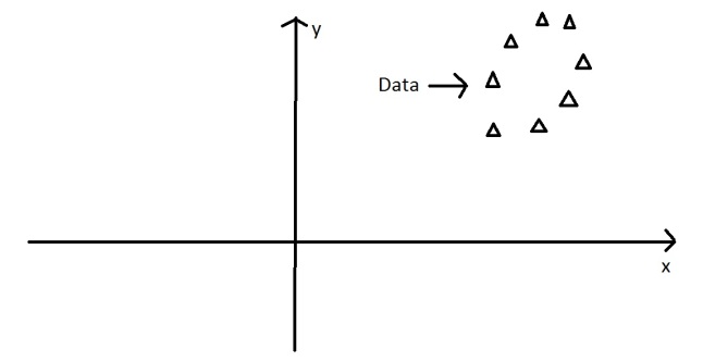
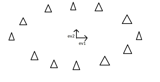
It is often useful to measure data in terms of its principal components rather than on a normal x-y axis. So what are principal components then? They’re the underlying structure in the data. They are the directions where there is the most variance, the directions where the data is most spread out. This is easiest to explain by way of example. Here’s some triangles in the shape of an oval:

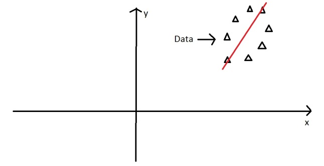
Imagine that the triangles are points of data. To find the direction where there is most variance, find the straight line where the data is most spread out when projected onto it. A vertical straight line with the points projected on to it will look like this:

The data isn’t very spread out here, therefore it doesn’t have a large variance. It is probably not the principal component.

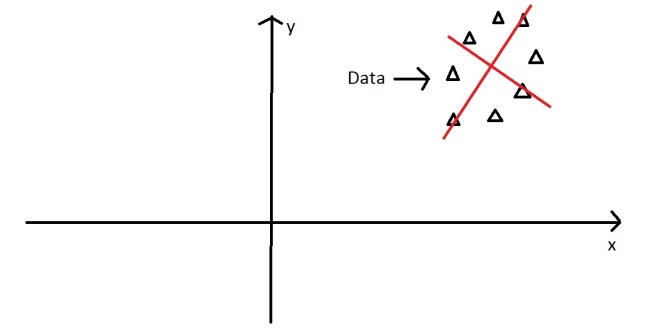
A horizontal line are with lines projected on will look like this:

On this line the data is way more spread out, it has a large variance. In fact there isn’t a straight line you can draw that has a larger variance than a horizontal one. A horizontal line is therefore the principal component in this example.

Luckily we can use maths to find the principal component rather than drawing lines and unevenly shaped triangles. This is where eigenvectors and eigenvalues come in.

Eigenvectors and Eigenvalues

When we get a set of data points, like the triangles above, we can deconstruct the set into eigenvectors and eigenvalues. Eigenvectors and values exist in pairs: every eigenvector has a corresponding eigenvalue. An eigenvector is a direction, in the example above the eigenvector was the direction of the line (vertical, horizontal, 45 degrees etc.) . An eigenvalue is a number, telling you how much variance there is in the data in that direction, in the example above the eigenvalue is a number telling us how spread out the data is on the line. The eigenvector with the highest eigenvalue is therefore the principal component.

Okay, so even though in the last example I could point my line in any direction, it turns out there are not many eigenvectors/values in a data set. In fact the amount of eigenvectors/values that exist equals the number of dimensions the data set has. Say i’m measuring age and hours on the internet. there are 2 variables, it’s a 2 dimensional data set, therefore there are 2 eigenvectors/values. If i’m measuring age, hours on internet and hours on mobile phone there’s 3 variables, 3-D data set, so 3 eigenvectors/values. The reason for this is that eigenvectors put the data into a new set of dimensions, and these new dimensions have to be equal to the original amount of dimensions. This sounds complicated, but again an example should make it clear.

Here’s a graph with the oval:

At the moment the oval is on an x-y axis. x could be age and y hours on the internet. These are the two dimensions that my data set is currently being measured in. Now remember that the principal component of the oval was a line splitting it longways:

It turns out the other eigenvector (remember there are only two of them as it’s a 2-D problem) is perpendicular to the principal component. As we said, the eigenvectors have to be able to span the whole x-y area, in order to do this (most effectively), the two directions need to be orthogonal (i.e. 90 degrees) to one another. This why the x and y axis are orthogonal to each other in the first place. It would be really awkward if the y axis was at 45 degrees to the x axis. So the second eigenvector would look like this:

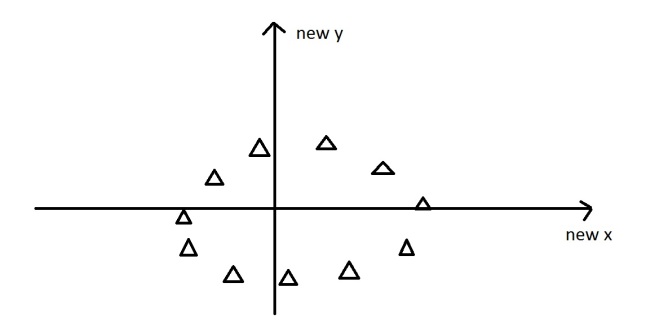
The eigenvectors have given us a much more useful axis to frame the data in. We can now re-frame the data in these new dimensions. It would look like this::

Note that nothing has been done to the data itself. We’re just looking at it from a different angle. So getting the eigenvectors gets you from one set of axes to another. These axes are much more intuitive to the shape of the data now. These directions are where there is most variation, and that is where there is more information (think about this the reverse way round. If there was no variation in the data [e.g. everything was equal to 1] there would be no information, it’s a very boring statistic – in this scenario the eigenvalue for that dimension would equal zero, because there is no variation).

But what do these eigenvectors represent in real life? The old axes were well defined (age and hours on internet, or any 2 things that you’ve explicitly measured), whereas the new ones are not. This is where you need to think. There is often a good reason why these axes represent the data better, but maths won’t tell you why, that’s for you to work out.

How does PCA and eigenvectors help in the actual analysis of data? Well there’s quite a few uses, but a main one is dimension reduction.

Dimension Reduction

PCA can be used to reduce the dimensions of a data set. Dimension reduction is analogous to being philosophically reductionist: It reduces the data down into it’s basic components, stripping away any unnecessary parts.

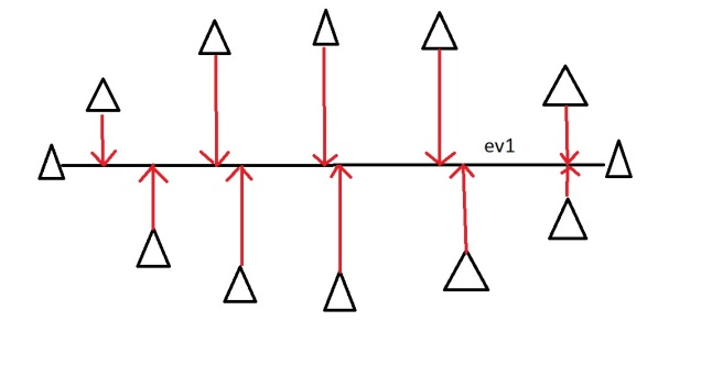
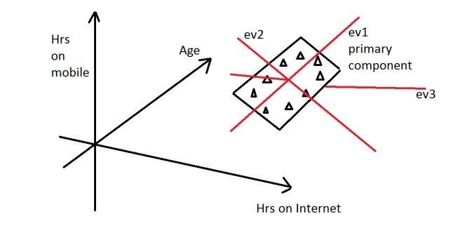
Let’s say you are measuring three things: age, hours on internet and hours on mobile. There are 3 variables so it is a 3D data set. 3 dimensions is an x,y and z graph, It measure width, depth and height (like the dimensions in the real world). Now imagine that the data forms into an oval like the ones above, but that this oval is on a plane. i.e. all the data points lie on a piece of paper within this 3D graph (having width and depth, but no height). Like this:

When we find the 3 eigenvectors/values of the data set (remember 3D probem = 3 eigenvectors), 2 of the eigenvectors will have large eigenvalues, and one of the eigenvectors will have an eigenvalue of zero. The first two eigenvectors will show the width and depth of the data, but because there is no height on the data (it is on a piece of paper) the third eigenvalue will be zero. On the picture below ev1 is the first eignevector (the one with the biggest eigenvalue, the principal component), ev2 is the second eigenvector (which has a non-zero eigenvalue) and ev3 is the third eigenvector, which has an eigenvalue of zero.

We can now rearrange our axes to be along the eigenvectors, rather than age, hours on internet and hours on mobile. However we know that the ev3, the third eigenvector, is pretty useless. Therefore instead of representing the data in 3 dimensions, we can get rid of the useless direction and only represent it in 2 dimensions, like before:

This is dimension reduction. We have reduced the problem from a 3D to a 2D problem, getting rid of a dimension. Reducing dimensions helps to simplify the data and makes it easier to visualise.

Note that we can reduce dimensions even if there isn’t a zero eigenvalue. Imagine we did the example again, except instead of the oval being on a 2D plane, it had a tiny amount of height to it. There would still be 3 eigenvectors, however this time all the eigenvalues would not be zero. The values would be something like 10, 8 and 0.1. The eigenvectors corresponding to 10 and 8 are the dimensions where there is alot of information, the eigenvector corresponding to 0.1 will not have much information at all, so we can therefore discard the third eigenvector again in order to make the data set more simple.

Example: the OxIS 2013 report

The OxIS 2013 report asked around 2000 people a set of questions about their internet use. It then identified 4 principal components in the data. This is an example of dimension reduction. Let’s say they asked each person 50 questions. There are therefore 50 variables, making it a 50-dimension data set. There will then be 50 eigenvectors/values that will come out of that data set. Let’s say the eigenvalues of that data set were (in descending order): 50, 29, 17, 10, 2, 1, 1, 0.4, 0.2….. There are lots of eigenvalues, but there are only 4 which have big values – indicating along those four directions there is alot of information. These are then identified as the four principal components of the data set (which in the report were labelled as enjoyable escape, instrumental efficiency, social facilitator and problem generator), the data set can then be reduced from 50 dimensions to only 4 by ignoring all the eigenvectors that have insignificant eigenvalues. 4 dimensions is much easier to work with than 50! So dimension reduction using PCA helped simplify this data set by finding the dominant dimensions within it.

Principal Component Analysis 4 Dummies: Eigenvectors, Eigenvalues and Dimension Reduction

Near Wellbore Stresses

For a cylindrical hole in  in a thick, homogeneous, isotropic elastic plate subjected to effective minimum and maximum principal stresses ($\sigma _ H$ and $\sigma _h$),
the radial stress,

\[ \sigma_{t}^{'}=\frac{1}{2}\left(\sigma_{H}^{'}+\sigma_{h}^{'}\right)\left(1+\frac{r_{w}^{2}}{r^{2}}\right)-\frac{1}{2}\left(\sigma_{H}^{'}-\sigma_{h}^{'}\right)\left(1+\frac{3r_{w}^{4}}{r^{4}}\right)\cos2\theta-\frac{r_{w}^{2}}{r^{2}}\left(p_{w}-p_{r}\right)
\]


circumferential (hoop) stress,

\[ \sigma_{t}^{'}=\frac{1}{2}\left(\sigma_{H}^{'}+\sigma_{h}^{'}\right)\left(1+\frac{r_{w}^{2}}{r^{2}}\right)-\frac{1}{2}\left(\sigma_{H}^{'}-\sigma_{h}^{'}\right)\left(1+\frac{3r_{w}^{4}}{r^{4}}\right)\cos2\theta-\frac{r_{w}^{2}}{r^{2}}\left(p_{w}-p_{r}\right)
\]


tangential shear stress,

\[ \tau_{r\phi}=\frac{1}{2}\left(\sigma_{H}^{'}-\sigma_{h}^{'}\right)\left(1+\frac{2r_{w}^{2}}{r^{2}}-\frac{3r_{w}^{4}}{r^{4}}\right)
\]


Hoop stress analysis can be used to determine wellbore failures, breakouts and fracture.

Theses stress changes as the location moves away from wellbore.

• Kirsch, G., Die Theorie der Elastizitat und die Beaurforisse der Festigkeitslehre, VDI Z 1857 1968, 42, 707, 1898.
• Jaeger, J. C., Elasticity, Fracture and Flow, 212 pp., Methuen, London, 1961.
• Zoback, M. D., D. Moos, L. Mastin, and R. N. Anderson (1985), Well bore breakouts and in situ stress, J. Geophys. Res., 90(B7), 5523–5530, doi:10.1029/JB090iB07p05523.

Rock Brittleness

Definition:

• Brittle rocks undergo little or no ductile deformation past the yield point (or elastic limit) of the rock.
• Brittle rocks absorb relatively little energy before fracturing.
• Brittle rocks have a strong tendency to fracture.
• Brittle rocks have a higher angle of internal friction

Brittleness in Mining Industry:

Some authors in the mining industry define brittleness index B (loosely defined, but the concept is also called brittleness ratio, brittleness coefficient, or ductility number) as the ratio of uniaxial compressive strength to tensile strength.

\[ B = \frac{\mathrm{compressive}\ \mathrm{strength}}{\mathrm{tensile}\ \mathrm{strength}} = \frac{\sigma_\mathrm{C}}{\sigma_\mathrm{T}}
\]

Altindag (2003) also gives:

\[ B = \frac{\sigma_\mathrm{C} - \sigma_\mathrm{T}}{\sigma_\mathrm{C} + \sigma_\mathrm{T}} \]

Altindag (2002 and 2003) further showed that the most useful measure may be the mean average of compressive and tensile strength:

\[ B = \tfrac12 \times (\sigma_\mathrm{C} + \sigma_\mathrm{T})  \]

Tensile strength is usually correlated with compressive strength, and it may be possible to use just one of these measures as a proxy for brittleness. This is good, because some (most?) labs only measure compressive strength as a standard test, e.g. in routine triaxial rig tests.

Brittleness in Geophysics:

Rickman et al. 2008 proposed using Young's modulus E and Poisson's ratio ν to estimate brittleness. This is appealing to development geophyisicists because elastic moduli are readily available from logs and accessible from seismic data via seismic inversion. Two recent examples are Sharma & Chopra 2012 and Gray et al. 2012. Gray et al. gave the following equations for 'brittleness index' B:

\[ B=50\% \times \left(\frac{E_{\mathrm{min}}-E}{E_{\mathrm{min}}-E_{\mathrm{max}}}+\frac{\nu_{\mathrm{max}}-\nu}{\nu_{\mathrm{max}}-\nu_{\mathrm{min}}}\right) \]

However, this approach remains skeptical, which assumes that a shale's brittleness is (a) a tangible rock property and (b) a simple function of elastic moduli. Computing shale brittleness from elastic properties is not physically meaningful, stated by Lev Vernik stated at the SEG Annual Meeting in 2012.

http://subsurfwiki.org/wiki/Brittleness

Organic Nanopores in Shale

• Organic Nanopores Structure Materials - Pyrobitumen

The carbon-rich residue of catagenesis, pyrobitumen constitutes the material of organic part of the rock. The Pyrobitumen is a type of solid, amorphous organic matter, which is insoluble to organic solvent (different from bitumen). However, one should not confuse pyrobitumen with residual kerogen in a mature source rock and the distinction is based on microscopic evidence of fluid flow within the rock fabric and is usually not determined. The thermal processes (bitumen to pyrobitumen) driving the molecular cross-linking also decrease the atomic ratio of hydrogen to carbon from greater than one to less than one and ultimately to approximately one half.

• Gas Adsorption

Similar to surface tension, adsorption is a consequence of surface energy. In a bulk material, all the bonding requirements (be they ionic, covalent, or metallic) of the constituent atoms of the material are filled by other atoms in the material. However, atoms on the surface of the adsorbent are not wholly surrounded by other adsorbent atoms and therefore can attract adsorbates. The exact nature of the bonding depends on the details of the species involved, but the adsorption process is generally classified as physisorption (characteristic of weak van der Waals forces) or chemisorption (characteristic of covalent bonding). It may also occur due to electrostatic attraction.

Affecting Factors: (i) In general, easily liquefiable gases e.g., CO2, NH3, Cl2 and SO2 etc. are adsorbed to a greater extent than the elemental gases e.g. H2, O2, N2, He etc. (while chemisorption is specific in nature.) 

(ii) Porous and finely powdered solid e.g. charcoal, fullers earth, adsorb more as compared to the hard non-porous materials. Due to this property powdered charcoal is used in gas masks.

However, most importantly, the extent of adsorbate adsorption depends directly upon the surface area of the adsorbent.

Adsorption forces and potentials: Methane is generally considered as non-polar molecules. The inter-molecular forces between gas molecules and nanopore surface can be obtained using atom–atom pair potentials, namely a Lennard–Jones (LJ) potential.

[\V_{LJ} = 4\varepsilon \left[ \left(\frac{\sigma}{r}\right)^{12} - \left(\frac{\sigma}{r}\right)^{6} \right] = \varepsilon \left[ \left(\frac{r_{m}}{r}\right)^{12} - 2\left(\frac{r_{m}}{r}\right)^{6} \right]

\]

where ε is the depth of the potential well, σ is the finite distance at which the inter-particle potential is zero, r is the distance between the particles, and rm is the distance at which the potential reaches its minimum.

The r−12 term, which is the repulsive term, describes Pauli repulsion at short ranges due to overlapping electron orbitals and the r−6 term, which is the attractive long-range term, describes attraction at long ranges (van der Waals force, or dispersion force).

Isotherm models: Irving Langmuir was the first to derive a scientifically based adsorption isotherm in 1918. The model applies to gases adsorbed on solid surfaces. It is a semi-empirical isotherm with a kinetic basis and was derived based on statistical thermodynamics. It is the most common isotherm equation to use due to its simplicity and its ability to fit a variety of adsorption data. The mono-layer assumption is addressed by the BET isotherm for relatively flat (non-microporous) surfaces.

Surface Tension Change with Salinity

http://socratic.org/s/apAxrxjJ

Yes, adding salt to water does increase the surface tension of water, although not by any significant amount. 

It is a very common misconception that salt is a surfactant, i.e. a compound that either lowers or breaks surface tension. However, experiments done with salt water show that surface tension actually increases when salt is added to pure water. 

As you know, sodium chloride, or $NaCl$, is a strong electrolyte, which means it completely dissociates into sodium cations, $N{a}^{+}$, and chloride anions, $C{l}^{-}$, when placed in water.

http://chem.wisc.edu/deptfiles/genchem/sstutorial/Text7/Tx75/tx75.html

It turns out that the strong interactions between the sodium cations and the partial negative oxygen, and the chloride anions and the partial positive hydrogens, although they disrupt part of the hydrogen bonding that takes place between water molecules, actually strengthen the surface tension of water.

In other words, you get some ionic component to the overall hydrogen bond-dominated interactions from the addition of these cations and anions. 

A very common experiment meant to illustrate this concept is done by placing salt water drops on a penny. I'll post a link to a great article on such an experiment performed by Lucas Cherkewski

http://lucas.ecustom.ca/science-fair/

Statoil to build the world’s first floating wind farm: Hywind Scotland

Statoil has made the final investment decision to build the world’s first floating wind farm: The Hywind pilot park offshore Peterhead in Aberdeenshire, Scotland.

http://www.statoil.com/en/NewsAndMedia/News/2015/Pages/03Nov_HywindScotland_news_page.aspx