Monday, October 9, 2017

Viscoplasticity and

Viscoplasticity is a theory in continuum mechanics that describes the rate-dependent/time-dependent inelastic behavior of solids.

The inelastic behavior that is the subject of viscoplasticity is plastic deformation which means that the material undergoes unrecoverable deformations when a load level is reached. Rate-dependent plasticity is important for transient plasticity calculations. The main difference between rate-independent plastic and viscoplastic material models is that the latter exhibit not only permanent deformations after the application of loads but continue to undergo a creep flow as a function of time under the influence of the applied load.

The elastic response of viscoplastic materials can be represented in one-dimension by Hookean spring elements. Rate-dependence can be represented by nonlinear dashpot elements in a manner similar to viscoelasticity. Plasticity can be accounted for by adding sliding frictional elements as shown in Figure 1.[2] In the figure E is the modulus of elasticity, λ is the viscosity parameter and N is a power-law type parameter that represents non-linear dashpot [σ(dε/dt)= σ = λ(dε/dt)(1/N)]. The sliding element can have a yield stress (σy) that is strain rate dependent, or even constant, as shown in Figure 1c.


Viscoelasticity is the property of materials that exhibit both viscous and elastic characteristics when undergoing deformation. Viscous materials, like honey, resist shear flow and strain linearly with time when a stress is applied. Elastic materials strain when stretched and quickly return to their original state once the stress is removed.

Viscoelastic materials have elements of both of these properties and, as such, exhibit time-dependent strain. Whereas elasticity is usually the result of bond stretching along crystallographic planes in an ordered solid, viscosity is the result of the diffusion of atoms or molecules inside an amorphous material.[1]

Viscoplasticity
Viscoelasticity

Monday, July 24, 2017

PCA - Principal Component Analysis

Principal Component Analysis 4 Dummies: Eigenvectors, Eigenvalues and Dimension Reduction

Having been in the social sciences for a couple of weeks it seems like a large amount of quantitative analysis relies on Principal Component Analysis (PCA). This is usually referred to in tandem with eigenvalues, eigenvectors and lots of numbers. So what’s going on? Is this just mathematical jargon to get the non-maths scholars to stop asking questions? Maybe, but it’s also a useful tool to use when you have to look at data. This post will give a very broad overview of PCA, describing eigenvectors and eigenvalues (which you need to know about to understand it) and showing how you can reduce the dimensions of data using PCA. As I said it’s a neat tool to use in information theory, and even though the maths is a bit complicated, you only need to get a broad idea of what’s going on to be able to use it effectively.

There’s quite a bit of stuff to process in this post, but i’ve got rid of as much maths as possible and put in lots of pictures.

What is Principal Component Analysis?

First of all Principal Component Analysis is a good name. It does what it says on the tin. PCA finds the principal components of data.

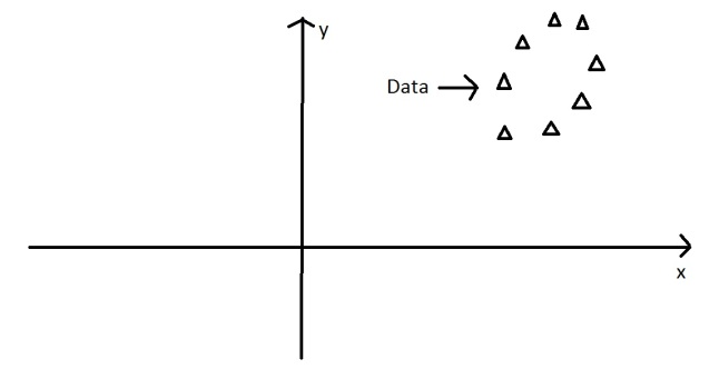
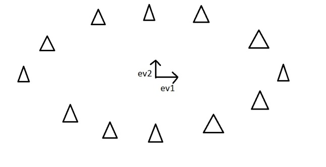
It is often useful to measure data in terms of its principal components rather than on a normal x-y axis. So what are principal components then? They’re the underlying structure in the data. They are the directions where there is the most variance, the directions where the data is most spread out. This is easiest to explain by way of example. Here’s some triangles in the shape of an oval:

PCA3

Imagine that the triangles are points of data. To find the direction where there is most variance, find the straight line where the data is most spread out when projected onto it. A vertical straight line with the points projected on to it will look like this:
PCA9

The data isn’t very spread out here, therefore it doesn’t have a large variance. It is probably not the principal component.

A horizontal line are with lines projected on will look like this:

PCA8

On this line the data is way more spread out, it has a large variance. In fact there isn’t a straight line you can draw that has a larger variance than a horizontal one. A horizontal line is therefore the principal component in this example.

Luckily we can use maths to find the principal component rather than drawing lines and unevenly shaped triangles. This is where eigenvectors and eigenvalues come in.


Eigenvectors and Eigenvalues

When we get a set of data points, like the triangles above, we can deconstruct the set into eigenvectors and eigenvalues. Eigenvectors and values exist in pairs: every eigenvector has a corresponding eigenvalue. An eigenvector is a direction, in the example above the eigenvector was the direction of the line (vertical, horizontal, 45 degrees etc.) . An eigenvalue is a number, telling you how much variance there is in the data in that direction, in the example above the eigenvalue is a number telling us how spread out the data is on the line. The eigenvector with the highest eigenvalue is therefore the principal component.

Okay, so even though in the last example I could point my line in any direction, it turns out there are not many eigenvectors/values in a data set. In fact the amount of eigenvectors/values that exist equals the number of dimensions the data set has. Say i’m measuring age and hours on the internet. there are 2 variables, it’s a 2 dimensional data set, therefore there are 2 eigenvectors/values. If i’m measuring age, hours on internet and hours on mobile phone there’s 3 variables, 3-D data set, so 3 eigenvectors/values. The reason for this is that eigenvectors put the data into a new set of dimensions, and these new dimensions have to be equal to the original amount of dimensions. This sounds complicated, but again an example should make it clear.

Here’s a graph with the oval:

PCA2

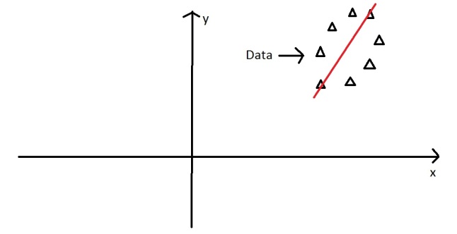
At the moment the oval is on an x-y axis. x could be age and y hours on the internet. These are the two dimensions that my data set is currently being measured in. Now remember that the principal component of the oval was a line splitting it longways:

PCA10
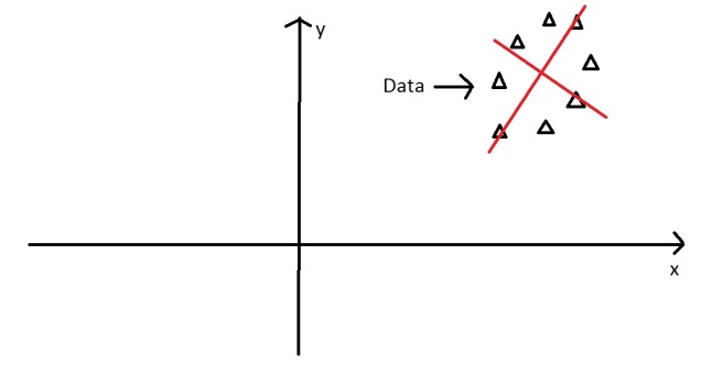
It turns out the other eigenvector (remember there are only two of them as it’s a 2-D problem) is perpendicular to the principal component. As we said, the eigenvectors have to be able to span the whole x-y area, in order to do this (most effectively), the two directions need to be orthogonal (i.e. 90 degrees) to one another. This why the x and y axis are orthogonal to each other in the first place. It would be really awkward if the y axis was at 45 degrees to the x axis. So the second eigenvector would look like this:
PCA11

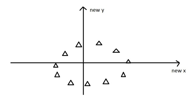
The eigenvectors have given us a much more useful axis to frame the data in. We can now re-frame the data in these new dimensions. It would look like this::

PCA1

Note that nothing has been done to the data itself. We’re just looking at it from a different angle. So getting the eigenvectors gets you from one set of axes to another. These axes are much more intuitive to the shape of the data now. These directions are where there is most variation, and that is where there is more information (think about this the reverse way round. If there was no variation in the data [e.g. everything was equal to 1] there would be no information, it’s a very boring statistic – in this scenario the eigenvalue for that dimension would equal zero, because there is no variation).

But what do these eigenvectors represent in real life? The old axes were well defined (age and hours on internet, or any 2 things that you’ve explicitly measured), whereas the new ones are not. This is where you need to think. There is often a good reason why these axes represent the data better, but maths won’t tell you why, that’s for you to work out.

How does PCA and eigenvectors help in the actual analysis of data? Well there’s quite a few uses, but a main one is dimension reduction.

Dimension Reduction

PCA can be used to reduce the dimensions of a data set. Dimension reduction is analogous to being philosophically reductionist: It reduces the data down into it’s basic components, stripping away any unnecessary parts.

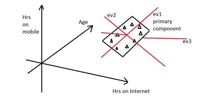
Let’s say you are measuring three things: age, hours on internet and hours on mobile. There are 3 variables so it is a 3D data set. 3 dimensions is an x,y and z graph, It measure width, depth and height (like the dimensions in the real world). Now imagine that the data forms into an oval like the ones above, but that this oval is on a plane. i.e. all the data points lie on a piece of paper within this 3D graph (having width and depth, but no height). Like this:

PCA12

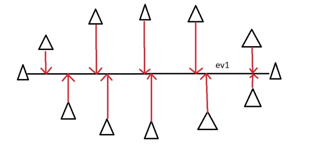
When we find the 3 eigenvectors/values of the data set (remember 3D probem = 3 eigenvectors), 2 of the eigenvectors will have large eigenvalues, and one of the eigenvectors will have an eigenvalue of zero. The first two eigenvectors will show the width and depth of the data, but because there is no height on the data (it is on a piece of paper) the third eigenvalue will be zero. On the picture below ev1 is the first eignevector (the one with the biggest eigenvalue, the principal component), ev2 is the second eigenvector (which has a non-zero eigenvalue) and ev3 is the third eigenvector, which has an eigenvalue of zero.

PCA13

We can now rearrange our axes to be along the eigenvectors, rather than age, hours on internet and hours on mobile. However we know that the ev3, the third eigenvector, is pretty useless. Therefore instead of representing the data in 3 dimensions, we can get rid of the useless direction and only represent it in 2 dimensions, like before:
PCA7

This is dimension reduction. We have reduced the problem from a 3D to a 2D problem, getting rid of a dimension. Reducing dimensions helps to simplify the data and makes it easier to visualise.

Note that we can reduce dimensions even if there isn’t a zero eigenvalue. Imagine we did the example again, except instead of the oval being on a 2D plane, it had a tiny amount of height to it. There would still be 3 eigenvectors, however this time all the eigenvalues would not be zero. The values would be something like 10, 8 and 0.1. The eigenvectors corresponding to 10 and 8 are the dimensions where there is alot of information, the eigenvector corresponding to 0.1 will not have much information at all, so we can therefore discard the third eigenvector again in order to make the data set more simple.

Example: the OxIS 2013 report

The OxIS 2013 report asked around 2000 people a set of questions about their internet use. It then identified 4 principal components in the data. This is an example of dimension reduction. Let’s say they asked each person 50 questions. There are therefore 50 variables, making it a 50-dimension data set. There will then be 50 eigenvectors/values that will come out of that data set. Let’s say the eigenvalues of that data set were (in descending order): 50, 29, 17, 10, 2, 1, 1, 0.4, 0.2….. There are lots of eigenvalues, but there are only 4 which have big values – indicating along those four directions there is alot of information. These are then identified as the four principal components of the data set (which in the report were labelled as enjoyable escape, instrumental efficiency, social facilitator and problem generator), the data set can then be reduced from 50 dimensions to only 4 by ignoring all the eigenvectors that have insignificant eigenvalues. 4 dimensions is much easier to work with than 50! So dimension reduction using PCA helped simplify this data set by finding the dominant dimensions within it.

Friday, February 24, 2017

Near Wellbore Stresses

For a cylindrical hole in  in a thick, homogeneous, isotropic elastic plate subjected to effective minimum and maximum principal stresses ($\sigma _ H$ and $\sigma _h$),
the radial stress,

\[ \sigma_{t}^{'}=\frac{1}{2}\left(\sigma_{H}^{'}+\sigma_{h}^{'}\right)\left(1+\frac{r_{w}^{2}}{r^{2}}\right)-\frac{1}{2}\left(\sigma_{H}^{'}-\sigma_{h}^{'}\right)\left(1+\frac{3r_{w}^{4}}{r^{4}}\right)\cos2\theta-\frac{r_{w}^{2}}{r^{2}}\left(p_{w}-p_{r}\right)
\]


circumferential (hoop) stress,

\[ \sigma_{t}^{'}=\frac{1}{2}\left(\sigma_{H}^{'}+\sigma_{h}^{'}\right)\left(1+\frac{r_{w}^{2}}{r^{2}}\right)-\frac{1}{2}\left(\sigma_{H}^{'}-\sigma_{h}^{'}\right)\left(1+\frac{3r_{w}^{4}}{r^{4}}\right)\cos2\theta-\frac{r_{w}^{2}}{r^{2}}\left(p_{w}-p_{r}\right)
\]


tangential shear stress,

\[ \tau_{r\phi}=\frac{1}{2}\left(\sigma_{H}^{'}-\sigma_{h}^{'}\right)\left(1+\frac{2r_{w}^{2}}{r^{2}}-\frac{3r_{w}^{4}}{r^{4}}\right)
\]


Hoop stress analysis can be used to determine wellbore failures, breakouts and fracture.


Theses stress changes as the location moves away from wellbore.


  • Kirsch, G., Die Theorie der Elastizitat und die Beaurforisse der Festigkeitslehre, VDI Z 1857 1968, 42, 707, 1898.
  • Jaeger, J. C., Elasticity, Fracture and Flow, 212 pp., Methuen, London, 1961.
  • Zoback, M. D., D. Moos, L. Mastin, and R. N. Anderson (1985), Well bore breakouts and in situ stress, J. Geophys. Res., 90(B7), 5523–5530, doi:10.1029/JB090iB07p05523.

Rock Brittleness

Definition:

  • Brittle rocks undergo little or no ductile deformation past the yield point (or elastic limit) of the rock.
  • Brittle rocks absorb relatively little energy before fracturing.
  • Brittle rocks have a strong tendency to fracture.
  • Brittle rocks have a higher angle of internal friction

Brittleness in Mining Industry:

Some authors in the mining industry define brittleness index B (loosely defined, but the concept is also called brittleness ratio, brittleness coefficient, or ductility number) as the ratio of uniaxial compressive strength to tensile strength.

\[ B = \frac{\mathrm{compressive}\ \mathrm{strength}}{\mathrm{tensile}\ \mathrm{strength}} = \frac{\sigma_\mathrm{C}}{\sigma_\mathrm{T}}
\]

Altindag (2003) also gives:

\[ B = \frac{\sigma_\mathrm{C} - \sigma_\mathrm{T}}{\sigma_\mathrm{C} + \sigma_\mathrm{T}} \]

Altindag (2002 and 2003) further showed that the most useful measure may be the mean average of compressive and tensile strength:

\[ B = \tfrac12 \times (\sigma_\mathrm{C} + \sigma_\mathrm{T})  \]

Tensile strength is usually correlated with compressive strength, and it may be possible to use just one of these measures as a proxy for brittleness. This is good, because some (most?) labs only measure compressive strength as a standard test, e.g. in routine triaxial rig tests.

Brittleness in Geophysics:

Rickman et al. 2008 proposed using Young's modulus E and Poisson's ratio ν to estimate brittleness. This is appealing to development geophyisicists because elastic moduli are readily available from logs and accessible from seismic data via seismic inversion. Two recent examples are Sharma & Chopra 2012 and Gray et al. 2012. Gray et al. gave the following equations for 'brittleness index' B:

\[ B=50\% \times \left(\frac{E_{\mathrm{min}}-E}{E_{\mathrm{min}}-E_{\mathrm{max}}}+\frac{\nu_{\mathrm{max}}-\nu}{\nu_{\mathrm{max}}-\nu_{\mathrm{min}}}\right) \]

However, this approach remains skeptical, which assumes that a shale's brittleness is (a) a tangible rock property and (b) a simple function of elastic moduli. Computing shale brittleness from elastic properties is not physically meaningful, stated by Lev Vernik stated at the SEG Annual Meeting in 2012.

Tuesday, December 1, 2015

Organic Nanopores in Shale


  • Organic Nanopores Structure Materials - Pyrobitumen

The carbon-rich residue of catagenesis, pyrobitumen constitutes the material of organic part of the rock. The Pyrobitumen is a type of solid, amorphous organic matter, which is insoluble to organic solvent (different from bitumen). However, one should not confuse pyrobitumen with residual kerogen in a mature source rock and the distinction is based on microscopic evidence of fluid flow within the rock fabric and is usually not determined. The thermal processes (bitumen to pyrobitumen) driving the molecular cross-linking also decrease the atomic ratio of hydrogen to carbon from greater than one to less than one and ultimately to approximately one half.


  • Gas Adsorption
Similar to surface tension, adsorption is a consequence of surface energy. In a bulk material, all the bonding requirements (be they ionic, covalent, or metallic) of the constituent atoms of the material are filled by other atoms in the material. However, atoms on the surface of the adsorbent are not wholly surrounded by other adsorbent atoms and therefore can attract adsorbates. The exact nature of the bonding depends on the details of the species involved, but the adsorption process is generally classified as physisorption (characteristic of weak van der Waals forces) or chemisorption (characteristic of covalent bonding). It may also occur due to electrostatic attraction.


Affecting Factors: (i) In general, easily liquefiable gases e.g., CO2, NH3, Cl2 and SO2 etc. are adsorbed to a greater extent than the elemental gases e.g. H2, O2, N2, He etc. (while chemisorption is specific in nature.) 

(ii) Porous and finely powdered solid e.g. charcoal, fullers earth, adsorb more as compared to the hard non-porous materials. Due to this property powdered charcoal is used in gas masks.

However, most importantly, the extent of adsorbate adsorption depends directly upon the surface area of the adsorbent.

Adsorption forces and potentials: Methane is generally considered as non-polar molecules. The inter-molecular forces between gas molecules and nanopore surface can be obtained using atom–atom pair potentials, namely a Lennard–Jones (LJ) potential.

[\V_{LJ} = 4\varepsilon \left[ \left(\frac{\sigma}{r}\right)^{12} - \left(\frac{\sigma}{r}\right)^{6} \right] = \varepsilon \left[ \left(\frac{r_{m}}{r}\right)^{12} - 2\left(\frac{r_{m}}{r}\right)^{6} \right]
\]


where ε is the depth of the potential well, σ is the finite distance at which the inter-particle potential is zero, r is the distance between the particles, and rm is the distance at which the potential reaches its minimum.

The r−12 term, which is the repulsive term, describes Pauli repulsion at short ranges due to overlapping electron orbitals and the r−6 term, which is the attractive long-range term, describes attraction at long ranges (van der Waals force, or dispersion force).

Isotherm models: Irving Langmuir was the first to derive a scientifically based adsorption isotherm in 1918. The model applies to gases adsorbed on solid surfaces. It is a semi-empirical isotherm with a kinetic basis and was derived based on statistical thermodynamics. It is the most common isotherm equation to use due to its simplicity and its ability to fit a variety of adsorption data. The mono-layer assumption is addressed by the BET isotherm for relatively flat (non-microporous) surfaces.

Sunday, November 22, 2015

Surface Tension Change with Salinity

Yes, adding salt to water does increase the surface tension of water, although not by any significant amount. 

It is a very common misconception that salt is a surfactant, i.e. a compound that either lowers or breaks surface tension. However, experiments done with salt water show that surface tension actually increases when salt is added to pure water. 

As you know, sodium chloride, or NaCl, is a strong electrolyte, which means it completely dissociates into sodium cations, Na+, and chloride anions, Cl, when placed in water.

http://chem.wisc.edu/deptfiles/genchem/sstutorial/Text7/Tx75/tx75.htmlhttp://chem.wisc.edu/deptfiles/genchem/sstutorial/Text7/Tx75/tx75.html

It turns out that the strong interactions between the sodium cations and the partial negative oxygen, and the chloride anions and the partial positive hydrogens, although they disrupt part of the hydrogen bonding that takes place between water molecules, actually strengthen the surface tension of water.

In other words, you get some ionic component to the overall hydrogen bond-dominated interactions from the addition of these cations and anions. 

A very common experiment meant to illustrate this concept is done by placing salt water drops on a penny. I'll post a link to a great article on such an experiment performed by Lucas Cherkewski

Tuesday, November 3, 2015

Statoil to build the world’s first floating wind farm: Hywind Scotland

Statoil has made the final investment decision to build the world’s first floating wind farm: The Hywind pilot park offshore Peterhead in Aberdeenshire, Scotland.

Sunday, September 20, 2015

Partnership to Take Rock-Fluid Research to the Atomic Level

A partnership between FEI Company and the University of Wyoming (UW) will enable for the first time ever the study of interactions between fluid and rocks at the atomic level for oil and gas research. The research – which aims to advance digital rock technology to achieve a better understanding of the fundamental forces at play in rock-fluid behavior – could potentially impact the entire oil and gas life cycle, from better well design for production to more effective enhanced oil recovery techniques for mature fields.

 - See more at: 
http://www.rigzone.com/news/oil_gas/a/140670/Partnership_to_Take_RockFluid_Research_to_the_Atomic_Level#sthash.wZ8dKwE6.dpuf

Wednesday, August 5, 2015

Mud to Lime: transitional lithotypes


Chalk vs Limestone vs Marble

Chalk is formed in a deep marine environment from the shells of microscopic algae which flourish near the surface, but die and fall to the seafloor. The kind of chalk used in old-style classrooms and lecture theatres scrapes off a thin layer of fine white dust as they are scraped over the abrasive surface of a "blackboard".

Limestone is formed in a shallower marine environment from the bodies of corals and shells, as well as the shells of microscopic sea life. Since it contains large lumps, it does not form such a fine white powder as chalk.

Marble is metamorphosed limestone, ie subjected to heat and pressure, the crystals grow and interlock, forming a stronger rock, more suitable for a building material. Sometimes minerals in the original limestone are still visible as swirls of colour in the marble.


Tuesday, July 7, 2015

Excel VBA

String:
  • chr(13) = change to the next line
  • _ =  break code to two lines


Function:

  • Transpose: Application.WorksheetFunction.Transpose()
  • Upper and lower bound: UBound() and LBound()
  • Join/concatenate: joins text, numbers, cell references, or a combination of those items into one text string
Range:
  • Range("B1:B10 , A4:D6").Select 选中两块不连续区域;
  • Range("B1:B10   A4:D6").Select 选中交叉的区域;
  • Range("B1:B10","A4:D6").Select 选中包含两块区域的最小矩形。


  • UsedRange: 所有使用过的单元格围成的区域;
  • Current Region: 所在的当前的区域;
  • Offset: 向下向右移动位置;
  • Range("A65536").End(xlUp).Offset(1,0): A列第一个非空的单元格;
  • Count: 单元格个数;
  • Address: 单元格位置;
  • Select, Activate
  • Clear, ClearContents, ClearComments, ClearFormats
  • Copy, Cut, Delete


Tuesday, June 30, 2015

Mudrock composition

Mudrocks, by definition, consist of at least fifty percent mud-sized particles. Specifically, mud is composed of silt-sized particles that are between 1/16 – 1/256 of a millimeter in diameter, and clay-sized particles which are less than 1/256 millimeter.

Mudrocks contain mostly clay minerals and quartz ($S_{i}O_{2}$)and feldspars (a group of minerals including aluminum silicates of soda (sodium oxide), potassium (potassium oxide), or lime (calcium oxide)). They can also contain the following particles at less than 63 micrometres: calcite ($CaCO_{3}$), dolomite ($CaMgCO_{3}$), siderite ($FeCO_{3}$), pyrite ($FeS_{2}$), marcasite ($FeS_{2}$), heavy minerals, and even organic carbon.

The term "mudrock" allows for further subdivisions of siltstone, claystone, mudstone, and shale. For example, a siltstone would be made of more than 50-percent grains that equate to 1/16 - 1/256 of a millimeter. "Shale" denotes fissility, which implies an ability to part easily or break parallel to stratification. Siltstone, mudstone, and claystone implies lithified, or hardened, detritus without fissility.

TypeMin grainMax grain
Claystone0 µm4 µm
Mudstone0 µm64 µm
Shale0 µm64 µm
Siltstone4 µm64 µm
Slatenana

Sunday, June 21, 2015

Turbulence Models

Turbulence:
Due to the high degree of mixing, turbulent flow exists. The heat and mass transfer rates are high and can not be explained by molecular transport only. It was seen as a random process in attempt to be specified in statistical parameters. Yet, it is not completely random.

Turbulence is normally expressed in terms of velocity. So there are extras terms in N-S equations, called Reynolds stress, described in terms of turbulence viscosity. This eddy viscosity is a strong function of the distance from the wall, where the eddy diminishes.

In turbulent flow, the kinetic energy imparted to the flow is dissipated into smaller eddies, and finally all the energy dissipated as thermal energy. Two sets of equations in CFD simulation are added to address the conservation of turbulence kinetic energy, $k$, and the turbulent energy dissipation rate, $\varepsilon$.

Prandtl Mixing Length:
When two eddies come closer, they are mixed. The mean distance between eddies is called the "mixing length", which analogous to the mean-free path in gases. The mixing length is a function of distance to the wall.

Friday, June 19, 2015

Model and Simulation: Laws of Conservation

Equation of Continuity:
For 2D incompressible fluid flow from mass conservation,

\[ \frac{\partial v_{x}}{\partial x}+\frac{\partial v_{y}}{\partial y}=0
\]

Thus,

\[ v_{y}=\int_{0}^{y}\frac{\partial v_{x}}{\partial x}dy
\]

Cauchy-Riemann Equation:
Define velocity by new variables, $Psi$, stream function and $phi$, velocity potential,

\[ v_{x}=-\frac{\partial\Psi}{\partial y}
\]

\[ v_{y}=\frac{\partial\Psi}{\partial x}
\]

\[ v_{x}=-\frac{\partial\phi}{\partial x}
\]

\[ v_{y}=-\frac{\partial\phi}{\partial y}
\]


An analytical function $w(z)$ of a complex variable, z, may be chosen such that

\[ w(z)=\phi(z)+i\Psi(z)
\]

satisfying above equations. Velocities can be obtained as the real and imaginary parts of the equation,

\[ \frac{dw}{dz}=-v_{x}+iv_{y}
\]

Equations of continuity, stream function and velocity function in different coordinates are shown below.


Navier-Stokes Equations:
Momentum transport:
\[ \rho\left(\frac{\partial v_{x}}{\partial t}+v_{x}\frac{\partial v_{x}}{\partial x}+v_{y}\frac{\partial v_{x}}{\partial y}+v_{z}\frac{\partial v_{x}}{\partial z}\right)=-\frac{\partial p}{\partial x}+\mu\left[\frac{\partial^{2}v_{x}}{\partial x^{2}}+\frac{\partial^{2}v_{x}}{\partial y^{2}}+\frac{\partial^{2}v_{x}}{\partial z^{2}}\right]+\rho g_{x}
\]

\[ \rho\left(\frac{\partial v_{y}}{\partial t}+v_{x}\frac{\partial v_{y}}{\partial x}+v_{y}\frac{\partial v_{y}}{\partial y}+v_{z}\frac{\partial v_{y}}{\partial z}\right)=-\frac{\partial p}{\partial y}+\mu\left[\frac{\partial^{2}v_{y}}{\partial x^{2}}+\frac{\partial^{2}v_{y}}{\partial y^{2}}+\frac{\partial^{2}v_{y}}{\partial z^{2}}\right]+\rho g_{y}
\]

\[ \rho\left(\frac{\partial v_{z}}{\partial t}+v_{x}\frac{\partial v_{z}}{\partial x}+v_{y}\frac{\partial v_{z}}{\partial y}+v_{z}\frac{\partial v_{z}}{\partial z}\right)=-\frac{\partial p}{\partial z}+\mu\left[\frac{\partial^{2}v_{z}}{\partial x^{2}}+\frac{\partial^{2}v_{z}}{\partial y^{2}}+\frac{\partial^{2}v_{z}}{\partial z^{2}}\right]+\rho g_{z}
\]

Chemical species in incompressible fluids:
\[ \rho\left(\frac{\partial C_{A}}{\partial t}+v_{x}\frac{\partial C_{A}}{\partial x}+v_{y}\frac{\partial C_{A}}{\partial y}+v_{z}\frac{\partial C_{A}}{\partial z}\right)=D_{AB}\left[\frac{\partial^{2}C_{A}}{\partial x^{2}}+\frac{\partial^{2}C_{A}}{\partial y^{2}}+\frac{\partial^{2}C_{A}}{\partial z^{2}}\right]-r_{A}

\]

Heat transfer:
\[ \rho\left(\frac{\partial T}{\partial t}+v_{x}\frac{\partial T}{\partial x}+v_{y}\frac{\partial T}{\partial y}+v_{z}\frac{\partial T}{\partial z}\right)=k\left[\frac{\partial^{2}T}{\partial x^{2}}+\frac{\partial^{2}T}{\partial y^{2}}+\frac{\partial^{2}T}{\partial z^{2}}\right]-\triangle H_{rxn}
\]

1D momentum balance for an unsteady state model gives,
\[ \rho\left(\frac{\partial v_{x}}{\partial t}+v_{x}\frac{\partial v_{x}}{\partial x}\right)=-\frac{\partial p}{\partial x}+\mu\left[\frac{\partial^{2}v_{x}}{\partial x^{2}}+\frac{\partial^{2}v_{x}}{\partial y^{2}}\right]+\rho g_{x}
\]


Using the incompressible fluid solution of equation of continuity,
\[ \rho\frac{\partial v_{x}}{\partial t}=-\frac{\partial p}{\partial x}+\mu\frac{\partial^{2}v_{x}}{\partial y^{2}}+\rho g_{x}

\]

The solution of 1D model equations are given below.


Boundary Conditions:
Differential equations of second order in spatial coordinates and first order in time require two boundary conditions and one initial condition to describe the system.

BC of the first kind:
The temperature or concentration of chemical species are specified at boundaries. This is also known as Dirichlet condition.

BC of the second kind:
The heat transfer or mass transfer flux is constant, also known as Neumann condition.

\[ q=-k_{f}\frac{\partial T}{\partial x}\mid_{x=0}
\]


BC of the third kind:
The flux is not constant, but the transfer coefficient is constant. Usually described in terms of heat or mass transfer coefficient.

\[ -k_{f}\frac{\partial T}{\partial x}\mid_{x=0}=h(T_{s}-T_{\infty})
\]


Friday, June 12, 2015

Model and Simulation: Physical Laws

Equation of State:
Ideal gas: $pV = RT$
Real gas: Peng-Robinson EOS
\[ p=\frac{RT}{(V-b)}-\frac{\alpha a}{V^{2}+2Vb-b^{2}}
\]

$ a = \frac{0.457235\,R^2\,T_c^2}{p_c} $
$ b = \frac{0.077796\,R\,T_c}{p_c} $
$ \alpha = \left(1 + \kappa \left(1-T_r^{\,0.5}\right)\right)^2 $
$ \kappa = 0.37464 + 1.54226\,\omega - 0.26992\,\omega^2 $
$ T_r = \frac{T}{T_c} $

In terms of compressibility, $Z=PV/(RT)$,  and in polynomial form:

$ A = \frac{a\alpha p}{ R^2\,T^2} $
$ B = \frac{b p}{RT} $
$ Z^3 - (1-B)\ Z^2 + (A-2B-3B^2)\ Z -(AB-B^2-B^3) = 0 $

where $\omega$ is the acentric factor of the species, R is the universal gas constant. Possible roots, 1 three real roots (largest, gas volume; smallest liquid volume); 2 one real (true volume) two imaginary.

The fugacity of pure component is given by,

\[ \ln\phi=\ln\frac{f}{p}=Z-1-\ln(Z-B)-\frac{A}{2\sqrt{2}B}\ln\left(\frac{Z+2.414B}{Z-0.414B}\right)

\]

Mixing rules:
Parameters of PR equation for the mixture of N simple fluids where molar percent of the i-th component is zi are defined by mixing rules

\[ a=\sum_{i}\sum_{j}z_{i}z_{j}a_{ij}
\]

\[ b=\sum_{i}z_{i}b_{i}
\]

where, $a_{ij}=(1-\delta_{ij})\sqrt{a_{i}a_{j}}$

Here aij is expressed through empirically determined binary interaction coefficient δij characterizing the binary formed by component i and component j.

Some δij are tabulated (e.g. table 4.2 in Pedersen and Christensen(2006)). For those one which are not tabulated formula of Chueh and Prausnitz (1967) could be used:

\[ 1-\delta_{ij}=\sqrt{\frac{2V_{c,i}^{1/6}V_{c,j}^{1/6}}{V_{c,i}^{1/3}V_{c,j}^{1/3}}}
\]


Formula for fugacity coefficient of the mixture, calculated via PR equation and standard mixing rules, has expression (see Peng and Robinson (1976) or equation 4.65 in Pedersen and Christensen (2006) for more detail)

\[ \ln\phi_{i}=\ln\frac{f_{i}}{z_{i}p}=\frac{b_{i}}{b}(Z-1)-\ln(Z-B)-\frac{A}{2\sqrt{2}B}\left(\frac{2}{a}\sum_{j}^{N}z_{j}a_{ij}-\frac{b_{i}}{b}\right)\ln\left(\frac{Z+2.414B}{Z-0.414B}\right)
\]

The enthalpy departure of the a fluid is given by,

\[ H-H^{*}=RT(Z-1)+\frac{T\frac{da}{dT}-a}{2\sqrt{2}b}\ln\left(\frac{Z+2.414B}{Z-0.414B}\right)
\]


Henry's Law:
The mole fraction or partial pressure of ith component, $p_i$ is proportional to the mole fraction of ith component in the liquid phase, $x_i$,

\[ p_{i}=H_{i}x_{i}
\]

For ideal gas,

\[ p_{i}=y_{i}P
\]


Thus, a linear equilibrium relationship is obtained,

\[ \frac{y_{i}}{x_{i}}=\frac{H_{i}}{P}
\]

For pure gas adsorption at pressure P, the number of moles adsorbed on the surface, n, is given by Henry's law for adsorption,

\[ n=kP
\]


$H_i$ is Henry constant; $P$ is total pressure; $y_i$ is mole fraction of ith component in vapor phase.

Newton's Law of Viscosity:
The shear stress is proportional to shear rate,

\[ \tau_{yx}=-\mu\frac{dv_{x}}{dy}

\]

All the gases and liquids and solutions of low-molecular-weight compounds exhibit Newtonian behavior. Non-Newtonian behaviors are shown below,


Some dimensionless numbers, such as Prandtl and Schmidt numbers can be obtained for empirical correlations for heat and mass transfer.

Fourier's Law:
Heat transfer rate of conduction due to temperature difference is written as,

\[ \dot{q}=kA\frac{(T_{2}-T_{1})}{\triangle z}=-kA\frac{dT}{dz}

\]

The differentiation form may be used if heat transfer area is a variable,

\[ \frac{d}{dz}\left(A\frac{dT}{dz}\right)=0

\]

Convective heat transfer at low temperature by Newton's law of cooling,

\[ \dot{q} = hA(T_2 - T_1)
\]

$k$ is the thermal conductivity; and $h$ is the heat transfer coefficient.

Fick's First Law:
For steady-state diffusion without convection, Fick's first law applies. The molar flux is described as,

\[ J_{A}=-CD_{AB}\nabla x_{A}\underrightarrow{C\,is\,constant}-D_{AB}\nabla C_{A}\underrightarrow{1-D}-D_{AB}A\left(\frac{dC_{A}}{dz}\right)

\]


where, $D_{AB}$ is the diffusion coefficient of A in B; $J_A$ is the molar flux of A; $C_A$ is the molar concentration of A; $x_A$ is the mole fraction of A.

Or the Fick's law gives the diffusive flux relative to the average velocity of fluid mixture. In absence of convection, the diffusive flux and the total flux are the same. For diffusion relative to fixed/stationary coordinates, the molar flux becomes,

\[ N_{A}=J_{A}+vC_{A}=-C_{A}D_{AB}\nabla x_{A}+v^* C_{A}
\]

where, average velocity, $v^*$ is $x_A v_A + x_B*v_B$.

\[ N = N_A + N_B = Cv^* = C_A v_A + C_B v_B
\]

Since the mass transfer results in some amount of convection (diffusional flux), the first law is valid only for dilute solutions or in cases of diffusion in solids. In concentrated solutions, the diffusion coefficient depends on the concentration.

Fick's Second Law:
It describes how diffusion causes the concentration to change with time.

\[ \frac{\partial C}{\partial t}=D_{AB}\frac{\partial C^{2}}{\partial z^{2}}

\]

Film Model:
The assumptions for film theory:
  1. The entire variation of concentration or temperature takes place within a thin fluid film adjacent to the interface. While, in the bulk fluid, the concentration or temperature is almost uniform.
  2. Within the film, the mass or heat transfer takes place by steady-state 1-D diffusion or conduction, respectively.
The mass transfer flux for species A is written in terms of diffusion coefficient, concentrations at the two faces of the fictitious film and film thickness,

\[ N_{A}=D_{AB}\frac{\left(C_{A2}-C_{A1}\right)}{\delta_{m}}

\]

Note that $C_{A2}$ is same as the concentration in bulk flow.

But in terms of mass transfer rate, $k$, which is measurable by experiment,

\[ N_{A}=k(C_{A2}-C_{A1})

\]

Differently, the mass transfer coefficient depends on the hydrodynamics, i.e. the fluid flow field in the bulk fluid.

Thus, the film thickness can be obtained,

\[ \delta_{m}=\frac{D_{AB}}{k}

\]

Two-Film Theory:
For two-phase flow, the mass transfer across the interface can be simplified:

  1. The resistance to mass transfer lies in two different fictitious films adjacent to the interface on both of its sides.
  2. The concentration of the chemical species in both phase at the interface is in equilibrium (insignificant mass transfer across the interface).

The total mass transfer coefficients $K_g$ and $K_l$ can be expressed in term of the individual mass transfer coefficient (when Henry's law applies):

\[ \frac{1}{K_{g}}=\frac{1}{k_{g}}+\frac{H}{k_{l}}
\]

\[ \frac{1}{K_{l}}=\frac{1}{k_{l}}+\frac{1}{Hk_{g}}

\]

If the mass transfer in the liquid phase is controlling, then kg>>kl and hence $K_l=k_l$. Vice versa.

Similarly, this also applies to heat transfer, where constant temperatures are canceled.

\[ \frac{1}{U}=\frac{1}{h_{1}}+\frac{1}{h_{2}}
\]


Arrhenius' Law:
The chemical reaction rate can be the product of two terms, one depends on concentration (associated with pressure terms) and one depends on temperature only.

\[ -r_{A}=f\left(C_{A},C_{B},...\right)k^{'}(T)
\]

The temperature term can be written as follows, Arrhenius' Law,
\[ k^{'}(T)=k_{0}^{'}e^{-E/RT}
\]

$k^{'}$ is the kinetic rate expression; $k_0^{'}$ is the constant, E is the activation energy of the reaction.

Adsorption Isotherms:
The equilibrium relationship relating $q$ (the mount adsorbed on the solid) and $C_A$ (the concentration of the adsorbate in the fluid)  is known as Isotherm. Sometimes, isotherms are given in terms of $K = K_a / K_d$ (rates of adsorption and desorption) and $\theta = q / q_0$ ($q_0$ is the adsorption capacity of adsorbent). Commonly used adsorption isotherms are,


  • Langmuir (1918), no interaction between the adsorbed molecules

\[ p=\frac{1}{K}\left(\frac{\theta}{1-\theta}\right)
\]
  • Brunauer-Emmett-Teller (1938), $p_{r}=p/p_{s}$, $q_m$ = constant
\[ \frac{q}{q_{m}}=\frac{K_{B}p_{r}}{(1-p_{r})(1-p_{r}+K_{B}p_{r})}
\]

  • Freundlich (1926) Empirical

\[ q=k_{F}C^{1/n_{F}}

\]

  • Raddke and Prausnitz (1972) combines Freundlich isotherms and Henry's law

\[ q=\frac{1}{\left(\frac{1}{K_{Hp}}+\frac{1}{k_{F}p^{1/n_{F}}}\right)}

\]

References:
Verma, Ashok Kumar. 2014. Process Modelling and Simulation in Chemical, Biochemical and Environmental Engineering. CRC Press.

http://en.wikipedia.org/wiki/Equation_of_state

http://kshmakov.org/fluid/note/3/

Wednesday, June 10, 2015

Model and Simulation: Simplifications in Model

Model Simplification:

Continuum: Laws of conservation hold in continuous phase. For dispersed bubble or solid particles in liquid, if the main mechanism is away from the interface of the dispersed and continuous phases, it may be convenient to consider the entire dispersion to be a continuous phase, e.g. study on the pipe wall and pressure loss. If the main mechanism takes place at the gas-liquid interface, continuum is meaningless, e.g. mass transfer between the bubble and liquid.

Combining simple and rigorous models: Two ways to model dispersed bubble in liquid, 1. build rigorous cell model for the dispersed bubble and surrounding liquid, and combine them in a simple manner. 2. Apply simple thin film model at the surface of the bubble and combine with the mass transfer and bubble-size distribution in a rigorous manner.

Uniform Probability Distribution: Useful in averaging the properties assuming the individual entity follow uniform distribution law, e.g. in adsorption, the probability of occupying the empty space on the surface is the same.

Parallel Mechanisms: The mechanism of  heat transfer is conduction, convection and radiation due to molecular motion, bulk flow and infrared radiation. The parallel mechanism allows us to treat different mechanisms separately, but under the assumption that there is no interaction between different mechanisms.

Analogy to Electrical Circuits: Many transport mechanisms are analog to the flow of current in electrical circuits.
Current flow: Ohm's Law;
Heat transfer: Fourier's Law;
Mass transfer: Fick's Law.
(Heat transfer due to radiation is described by Stephan-Boltzman's Law, i.e., the rate of heat transfer is proportional to the difference of the fourth power of the temperature.)

Film Model and Boundary Layer Approximation: The film model uses the assumption that in the small region adjacent to the wall, the variation is much larger than that at the center. Thus the concept of thin film at the wall is developed and accounts for all the variations. The central cylinder is considered with no variation.
But the boundary layer model allows the layer thickness to vary with time and distance. It is more likely an approximation to the reality, the experimental results.

Order of magnitude Approximation: If the ratio of the contribution from one mechanism and that from others is high enough, then the other mechanisms can be neglected to reduce the complexity.

Quasi-Steady State: The assumption for unsteady-state problem, that during a small time interval, the process is at steady-state is known as "quasi-steady state".

Finite and infinite dimensions: Many mathematical equations approach certain value when one or some of its parameters goes to infinity or zero, which is not possible in physical experiments. Thus, it can be assumed that when the parameter value is large or small enough, it is close to infinity or zero.

References:
Verma, Ashok Kumar. 2014. Process Modelling and Simulation in Chemical, Biochemical and Environmental Engineering. CRC Press.

Tuesday, June 9, 2015

Model and Simulation: Equations

Equations describe the interrelations between various parameters.

Algebraic Equation:

  • Linear equation, solved by matrix inversion
  • Non-linear equation, solved by linearisation or non-linear optimization

A non-linear equation $ F(\vec{x})=\vec{0}$ can be written by

\[ F(\vec{x})=\vec{R}
\]

where, $\vec{x}$, $\vec{0}$ and $\vec{R}$ are vectors.

R are the residuals and the objective function becomes $|\vec{R}|$, which is to be minimized.

By linearisation, the set of non-linear equations can be converted to,

\[ F_{i}(\vec{x})=-\sum_{j}J_{ij}(\vec{x})\triangle x_{j}
\]

where, $J_{ij}(\vec{x})=\frac{\partial F_{i}(\vec{x})}{\partial x}$.

An initial guess is required to start this iterative solving process. The Jacobian matrix is estimated using the values of x from the previous iteration until the right-hand side becomes less than the tolerance.

Various optimization methods can be used to search the optima within a given range. The problems can be

  1. The obtained optima is local optima or there are multiple optima -- Genetic Algorithm, Simulated Annealing
  2. The solution won't converge or stick at particle values -- try different methods or change the initial guess
Again, the choice of initial guess is very important.


Differential Equations:
If only one type of derivative is involve, the equation is called ODE, ordinary differential equation, as opposed to PDE, partial differential equation.

A Cauchy problem in mathematics asks for the solution of a partial differential equation that satisfies certain conditions which are given on a hypersurface in the domain. A Cauchy problem can be an initial value problem (given initial value, how the system evolves with time) or a boundary value problem (specifying the boundary condition instead), but it can be none of them. Cauchy boundary conditions require both the function value and normal derivative on the boundary of the domain (a Dirichlet and a Neumann boundary condition) to ensure a unique solution.

Sometimes, PDEs are converted into simultaneous ODEs or algebraic equations (a large system of coupled ODEs with derivatives with respect to time). When the phenomena vary with time, the spatial variables are discretised and time is considered a continuous variable. Such as parabolic and hyperbolic equations in unsteady-state models. This method is termed a "method-of-line".

In steady state models, spatial discretisation results in algebraic equations. Such as elliptic equations.


Differential-Algebraic Equations:

DAEs, these types of mixed equations contain unsteady-state material and energy balance equations, equilibrium relationships, consistency equations etc.


Other Equation Type Classification:

Homogeneous Function:
If x is the solution of the function, so is $\lambda x$.
\[ f(\lambda x)=\lambda^{n}f(x)
\]


Homogeneous linear differential equations:
 If  $\phi(x)$  is a solution, so is  $c \phi(x)$. In another word, each term in a linear differential equation must contain y or any derivative of y, such as $ \sin(x) \frac{d^2y}{dx^2} + 4 \frac{dy}{dx} + y = 0 $.

Second order differential equations:

\[ Au_{xx} + 2Bu_{xy} + Cu_{yy} + Du_x + Eu_y + F = 0
\]

If $B^2 - AC > 0$, hyperbolic partial differential equation;
If $B^2 - AC = 0$, parabolic PDE;
If $B^2 - AC < 0$, elliptic PDE.

The most famous wave equation is a hyperbolic PDE. In one spatial dimension, this is $u_{tt} - u_{xx} = 0$.

Source of Equations:
The source of the equations depends on the field of application and the knowledge of the modeler.

Empirical Equations:
These can be obtained by fitting the experimental data in terms of important parameters with somem simple functions. The relation can explicit or implicit (friction factor by McCable et al. 1993).

Based on theoretical concepts:
Such as the calculation/estimation of thermodynamic properties.

Consistency Equations:
Based on the fact that the fractional composition of each component should add up to 1, in terms of mole and mass.

Law of conservation:
Such as equation of continuity and the momentum-balance equation with considerations of energy/mass generation or depletion in chemical reaction, viscous dissipation, electrical or electrochemical effects on the flow and other phenomena. The generalized equation of change is known as the Navier-Stokes equation.

Integration/Averaging:
Flow rate is obtained by integrating the velocity over the cross-sectional area;
Average velocity is then obtained by division of the total area.
Also, number-averaged particle diameter, porosity...

Population Balance:
Discrete event model considers the birth and death of population (breakage, agglomeration or coalescence).

References:
Verma, Ashok Kumar. 2014. Process Modelling and Simulation in Chemical, Biochemical and Environmental Engineering. CRC Press.

Monday, June 1, 2015

Models and Simulation - Types of Models

Types of Models:
Three major model types are deterministic model, discrete-event model and stochastic model.

  • Deterministic Models: No random variable;
  • Lumped Parameter Models: ODE, all spatial distributions are lumped into one variable;
  • Distributed Parameter Models: PDE, consisting of spatial derivatives;
  • Steady-State/Static Models: No temporal derivative;
  • Unsteady-State/Dynamic Models: With temporal derivatives;
  • Stochastic Models: Random variables involved (probability distribution function/pseudo-random numbers)
  • Population Balanced Models: In multiphase system, discrete/dispersed phases are present as particles, droplets or bubbles. Similar to the "birth and death" of individuals, the particles can agglomerate or break and the bubbles and droplets can break and coalesce. Thus, the number of identities of discrete phases, called population, and the size of the individuals change and form a particle/droplet/bubble-size distribution.
  • Agent-Based Models: Each part of the model , called an agent, is capable of making decisions with strong human behavior involved;
  • Discrete-Event Models: The states, even time, are considered discrete and NON-continuous;
  • Artificial Neural Network-based Models: A black-box approach to correlate various parameters and then predict outcomes from information available. No exact relation between the inputs and outputs is almost possible to establish. No contribution to the understanding of the phenomena.
  • Fuzzy Models: based on fuzzy mathematics or fuzzy logic involving fuzzy variables. Fuzzy, not well quantified, such as small, large, very large.


-- The general-purpose language/software can handle various types of models/problems, but require coding of the model equations using the syntax and semantics of the software. While, more dedicated software generates an appropriate set of models of equations for the users to use, but the scope is limited.

-- Stochastic Models:
The random numbers are characterized by their moment. The first moment is known as "average" or "expectation". A model may consider only average properties, thus avoiding the complexity of the process due to the randomness of the properties. Many models consider random behavior of the parameters, although the outputs of the model are average properties. These models also are probabilistic in nature. Various moments of the random variables may be determined analytically (Coulomb's Law?) or by Monte Carlo simulation. The random variables follow a probability distribution function. The choice of the distribution is determined from the assumption involved.

References:
Verma, Ashok Kumar. 2014. Process Modelling and Simulation in Chemical, Biochemical and Environmental Engineering. CRC Press.

Friday, May 15, 2015

Osmotic Pressure Calculation

By thermodynamics, the chemical potential of solvent (water) in a solution containing pure solvent and solute is expressed as,

\[ \mu_{w}\left(l,x_{w},p+\pi\right)=\mu_{w}^{0}\left(l,p+\pi\right)+\nu RT\ln a_{w}
\]

where, $\mu_w$ is the chemical potential of solvent, which is a function of solvent, $l$, mole fraction of solvent $x_w$, external pressure, $p$, and additional osmotic pressure exerted by solutes, $\pi$ (whereas, for the pure solvent, $x_w$ goes away); $\nu$ is the dissociation coefficient (a solute dissociates into $\nu$ ions); $R$ is the gas constant; $T$ is temperature in consistent with $R$; $a_w$ is water activity.

The addition to the pressure is expressed through the expression for the energy of expansion:

\[ \mu_{w}^{o}(l,p+\pi)=\mu_{w}^{0}(l,p)+\int_{p}^{p+\pi}V\mathrm{d}p
\]


where, $V$ is the molar volume of solvent.

To balance the chemical potentials of solvent for two solutions with and without solute separated by semipermeable membrane, $\mu_{w}\left(l,x_{w},p+\pi\right)$ and $\mu_{w}\left(l,p\right)$,

\[ -\nu RT\ln a_{w}=\int_{p}^{p+\pi}V\mathrm{d}p

\]

Thus, osmotic pressure is expressed as opposed to pure solvent (water), in which water activity is 1,

\[ \pi=-\nu RT/V\ln a_{w}

\]

Conventionally, the gradient of osmotic pressure is approximated using the concentration or the mass fraction of solute (salt). The derivation is shown as follows.

A definition of water activity is,

\[ a_{w}=l_{w}x_{w}=l_w(1-x_s)
\]


where, $l_w$ is activity coefficient; and $x_w$ is the mole fraction of water in aqueous fraction ($x_s=1-x_w$ is the mole fraction of solute). By Raoult's law, $l_w$ is usually approximated as unity in dilute solution.

Using Taylor series, $\ln l_w(1-x_s) \approx -x_s$.

Thus, the osmotic pressure becomes ($C$ is the molar concentration of solute),

\[ \pi=-\nu RT/V\ln a_{w} = \nu RT/V x_s = \nu RT C

\]


Also, the relation between the gradients of osmotic pressure and chemical potential is,

\[ \nabla\pi=-\frac{1}{V}\cdot\nabla\mu_{w}

\]

The relation between the gradient of osmotic pressure and the concentration or the mass fraction of solute (salt) becomes,

\[  \nabla\pi\approx\nu RT\nabla C=\nu RT\frac{\rho}{M_{s}}\nabla X
\]


where, $\rho$ is the solution density; $M_s$ is molar mass of solute; and $X$ is the mass fraction of solute.

Monday, March 23, 2015

Effects of Cryogenic Fluids as A Fracturing Fluid - T. Patterson defense

233 bans or severe hindrances in municipalities across US
See www.foodandwaterwatcj.org/water/fracking

Non-water-based fracking
1. Gelled liquid CO2 (Gupta, 1998)
2. Cryogenic (Grundman, 1998)